Complexity Matching: Cortical Dynamics as the Reflecting Pool of Our Auditory World

Abstract

Empirical studies in complexity matching have sought to measure coordination of complex signals. Here we review the historic relevance of what is meant as ‘complexity’ and how that was led to a measurement of coordination between coupled agents. Then the extension of complexity matching theory to psychological and cognitive sciences will be reviewed here. The methods used to capture complexity from signals in social interactions will be outlined to understand the strengths and limitations of the methodology. We then conclude with discussing how prior methodology and relevant work on studying structural resonance can help inform the endeavor of finding complexity matching of brain responses and auditory stimuli.   

Introduction

Throughout this paper the word ‘complexity’ will be used heavily, touching upon the diverse span of its use in the scientific literature. More often than many researchers like to admit, the use of the word reflects a confusing etymology in which it can be encountered in the wild as an interchangeable word for meaning ‘complicated’ or ‘not simple’. Before you encounter the pervasive use of ‘complex’ or ‘complexity’ in this paper, we will define what it means for cognitive scientists in reference to the general use of ‘complexity’ and connect that to the methodology for measuring such a phenomenon.

Complexity  

            So, what is complexity? Well, we can start by talking about what it is not. On the other side of the epistemic table exists reductionism. Rene Descartes, being a famous proponent of this way of knowing, emphasized that we can best understand the natural world by understanding the most irreducible, fundamental component of some natural structure. This Lego block like epistemology compartmentalized natural phenomena, in the hopes of finding the smallest foundational block from which all other blocks are made out of. In other words, if someone can find the smallest unit in a system and understand its structure, then we will be able to also understand the larger structure of which it composes. This works under the assumption that interaction between blocks of the system architecture only tell us about their association, disregarding that there is more to know about a system other than the sum of its parts. Not to mention that scientists eventually find more structure underneath the presumed foundational unit of study, much how the atom is now studied as a complex system of its own.  

            Conversely, the recognition of complexity in systems theory looks at the interaction of system components. Herbert Simon (1981) points out that the focus on component interaction gives rise to the emergence phenomena. Which, unlike reductionism, presents a case for the limitation of only looking at the sum of its parts. Mitchell (2009) references many natural systems as examples of emergence e.g., ant colonies, the immune system, the world wide web, economies, and of course the brain. Ants much like neurons, are simple and low-level components of their systems. On their own they demonstrate a limited behavioral capacity, but their coordinated interactions demonstrate behaviors not expected to arise from observing the individual components (Hofstadter, 1979).   

            The above-mentioned examples and descriptions of complexity have been under the umbrella of what is termed as ‘organized complexity’. Weaver (1948) explains that a system in which the component interactions are not random and correlated, define organization behind the system complexity. On the other hand, systems with a large number of components and random component interactions are defined as ‘disorganized complexity’. The systems we refer to in this paper, unless otherwise noted, will be of organized complexity. Once we can know whether a system is organized or not, one can also measure the correlated component interactions to get a measure of how it is organized. Simon (1981) first argued that these system organizations can be best described as types of hierarchies when it comes to organized complexity. There can be an explicitly described formal hierarchy, in which a level of a system has direct influence and control over sub-components. We can refer to government hierarchies in which command and rank directly shape the organization of the system. Although such systems exist, it is more common to encounter a system where the formal hierarchy definition is irrelevant. Hierarchy in the non-formal way simply refers to the embedded relationship of system components. Although such a definition may seem vague, it allows room for looking at component interactions that do not follow a top down control and can involve bidirectional influence in the hierarchy.

Hierarchical Temporal Structure  

A hierarchical systems organization can arise from the interaction of simple functions. A prime example of this comes from the 2-dimensional Ising model (Ising, 1925; Onsager, 1944; Kim, 2011). The Ising model is a classic example of self-organized criticality, in which the atomic spins and their neighbor interactions showed magnetic phase transitions to occur without explicitly programming them. A critical state from the Ising model shows long-range spatial correlations of atomic spins, meaning that the interactions from a section of the lattice can influence groups of atoms at longer distances. The hierarchy in this system does not come predefined in the same way that one might think of when thinking of a formal hierarchy such as a presidential cabinet. Instead, the dynamics of the atomic spins create correlations from their neighbor interactions that travels across the map and a hierarchy of magnetic interactions across space emerges. Similarly, Hierarchical Temporal Structure (HTS) refers to correlations of system component interactions over the time domain. The term (HTS) was coined in (Falk & Kello, 2017) to measure temporal variations of acoustic energy of infant directed speech and adult directed speech at multiple time scales. These time scales referred to the embedded hierarchical organization of linguistic units such as phonemes, syllables, phrases, and utterances. Moreover, the importance of the embedded organization in language has been comparatively studied in music as well in terms of syntactic organization. A shared relation between language and speech organization has led to studies finding meaningful similarities in neural processing. More specifically, syntactic processing in the brain shares the recognition the embedded relationship of both linguistic and musical units to parse the temporal variation of the signal (Patel, 2003). In Cognitive Science, the focus on time domain measurements comes paired with the dynamical & complex systems approach. Simply put, a dynamical system consists of a state space whose trajectory over time is defined by a dynamical rule. This contrast classic symbolic and connectionist approaches that would focus on the representational content of states and the underlying mechanisms that would generate them. A focus on the state space trajectories also allows for the study of external and internal influences of the system, which in the Cognitive Science literature has been used to combine approaches of embodiment (Beer, 2000).     

            In this paper we review how the theoretical frames of complexity and dynamical systems have been extended in empirical work to develop methods for measuring the coupling of complex systems. The focus will primarily surround empirical work of speech and music as well as other signals seen in social interaction. We bring in current work pointing at the resonance of HTS from these signals e.g., phonetic levels in speech, seen in brain responses. From such work, we propose what it means to have coupling of complex stimuli and brain responses, along with the importance of structural resonance of these signals and what an empirical method would need to consider to successfully measure it. 

Coupled Behaviors

A dynamic systems approach on coupling can be traced back to the field of Synergetics, originated by Hermann Haken. Synergetics looked at how a system’s activity evolved over time as described by either external or internal control parameters. An example of external control parameters can be seen in the power input of a gas laser into an electrical current which modulates the rate of change of phase-locked activity. On the other hand, human hormones and neurotrasmitter activity has been modeled as having internal control parameters arising from their correlated interactions (Haken, 1969; Haken & Graham 1971). The latter example is akin to self-organization and the emergence phenomena, where the meaningful coupling of component behavior gives rise to the control parameters that best describe the dynamics of the system. Principles of Synergetics applied to human behavior were initially popularized by Kelso’s work on the emergence of interlimb coordination. Briefly put, cross-correlation of cyclic limb movement demonstrated evidence for mutual-entrainment. Varying cycling frequencies between limbs were also able to demonstrate non-arbitrary, subharmonic relationships (Kelso, Holt, Rubin, & Kugler, 1981; Haken, Kelso, & Bunz, 1985). Such work allowed for the coordination of human behavior to be understood as an emergent process deriving from non-linear, limit cycle oscillatory dynamics. Later work by Schoner & Kelso (1988) formalize principles of emergence in non-equilibrium systems and their stochastic, non-linear temporal patterns to connect macroscopic behavior coordination to the microscopic. Setting a common language of temporal dynamics and coordination allowed for Cognitive Science to generalize the functionality of cognitive processes across scales of measurement. An example given central to our review is the connection between non-linear temporal dynamics of neural activity to social behavior. This paper provides further perspective on this concept through the proposal of studying the coupling of complex input stimuli signals and brain responses, but we first explain the historical progress of related coupled behaviors in the field.

            Following the momentum from the Synergetics work, researchers started to look at the coordination involved in synchronizing motor output with the temporal relationships of the environment. Such a focus of study came to be known as Sensory-Motor-Synchronization (SMS) and combined behavioral experiments like the pervasive finger-tapping paradigm to the more recent neural activity focused designs (Iversen & Balasubramaniam, 2016). Insights from finger-tapping experimental paradigms have shown there to be a non-trivial synchrony, even when participants are told to match their tapping to a set of regular auditory beeps. The foundational work of SMS claims that such a process shows evidence for anticipatory processes. The regulatory activity of the coordinated synchrony therefore being controlled by phase and period correction (Repp, 2005; Repp & Su, 2013). Work in SMS have traditionally been able to demonstrate a strong advantage for auditory stimuli (McAuley & Henry, 2010; Patel, Iversen, Chen, & Repp, 2005). New work has been able to challenge the simple assumption that SMS has modality specific biases by showing how a tuning in stimuli presentation can illicit stronger responses from participants. Meaning that the presentation that works for one modality may not be balanced if directly transferred to another one (Gan, Huang, Zhou, Qian, & Wu, 2015; Hove, Iversen, Zhang, & Repp, 2013; John R Iversen, Patel, Nicodemus, & Emmorey, 2015). Furthermore, beat perception studies have shown anticipation as neural activity synchronization continues in the absence of an expected beat. Prediction models have established a link with the motor planning system as aiding with sensory prediction (Patel & Iversen, 2014). The signals of interest we review in this paper are auditory, aligning with the simple case for coordination in SMS.

            The anticipation work provided through the SMS framework was then taken a step further in what is termed as strong anticipation. Anticipation in the ‘weak’ sense, was defined as some system predicting future states to another system in which it needs to coordinate to (Dubois, 2003). For anticipation to be strong, the two systems in coordination are defined as making up a new whole system. This means that the lawful relationships between a system A and system B are coupled strongly enough where prediction of future states is not necessary, thus creating a new system C. Furthermore, because of such a strong coupling of the global dynamics of systems A & B, strong anticipation is measured by the coordination at multiple scales as opposed to a scale unit specific modulation as seen in SMS. Strong anticipation provides a framework for looking at coupling that does not necessitate internal representational models between coordinating systems. Instead, it looks at systems as being embedded in a hierarchical organization. In which both systems A & B can be observed as having their own identifiable properties, but through their interactions at multiple scales of measurement can define a higher-level system functionality (Stepp & Turvey, 2010). One of the first empirical examples for strong anticipation with the human perceptual system was a new take on the finger tapping experiments from SMS. Participants were instructed to synchronize their tapping to a chaotic metronome, which is not linearly predictable. Results showed that the functions of the fluctuations from the metronome and participants’ tapping had similar slopes, which provided evidence for the adherence to long-range correlations in signals (Stephen, Stepp, Dixon, & Turvey, 2008). Evidence for strong anticipation in interpersonal coordination has also been shown when participants coordinate pendulum swings. The series that coupled participants produced demonstrated correlations with their scaling exponent. Local, faster time-scale dependencies also were very limited in explaining the coordination. About ~30% of analyzed windows showed significant cross-correlation. This showed that although there may be some weak anticipation process involved, that it could not describe the behavior as a whole. The process for which strong anticipation is measured in interpersonal coordination was then dubbed as ‘complexity matching’ in this study, and it is the language that later studies use to describe similar scenarios (Marmelat & Delignières, 2012).

            The formal description for complexity matching came from the study of complex networks in the physics literature, in which the similarity of complexity between networks determines the extent of information exchange (West, Geneston, & Grigolini, 2008). Empirical adaptations to this concept were continued through the study of interpersonal coordination. Previous work assumed that global variability was solely responsible for complexity matching and that local interactions were primarily responsible for weak anticipation. To test this assumption, researchers use the same pendulum swing interpersonal coordination task but varied the uncoupled frequencies in dyads. This resulted in having more relative phase shifts acting as increased local corrections when the dissociation between dyad’s movement complexity increased (Fine, Likens, Amazeen, & Amazeen, 2015). Multi-fractal analyses have also been proposed to distinguish the matching attributed by local adjustments and the global statistical dynamics assumed by the prototypical complexity matching framework. Although results from multi-fractal methods allow for the distinction of local versus global matching, it does not discount local adjustments as being signs of weak anticipation but instead makes room for a combined approach of the behavior when doing complexity matching (Delignières, Almurad, Roume, & Marmelat, 2016). Furthermore, multi-fractal analyses have been used to present the argument for complexity matching methods being able to capture more ecologically valid data (Almurad, Roume, & Delignières, 2017). As we have referenced in this paper, the standard empirical framework for complexity matching has been in interpersonal coordination tasks. Moving away from movement data, a study tested for complexity matching between affiliative and argumentative dyadic conversations. They correlated their scaling functions from their produced signals, which in this case were speech. Results showed that there was more complexity matching between speech signals in affiliative conversations in comparison to argumentative (Abney, Paxton, Dale, & Kello, 2014). An extension of this approach sought to test whether complexity matching could happen in bilingual conversations. The experiment had bilingual participants (English & Spanish) engage in affiliative conversations under three conditions. The conditions had participants talk both in English, both in Spanish, or one in Spanish and the other in English. Results showed that complexity matching was seen with no significant difference across conditions, meaning that participants were able to converge their speak across languages and while speaking different languages. Further analyses also showed that there was also a matching of the lemmas of lexical words (lexical matching) across languages. The longer timescales of the scaling function from produced speech were shown to be the most relevant in complexity matching. With these results the authors found it clear to relate the matching observed to be related to a convergence of prosody i.e., the similarity in how informational linguistic units are organized. Which can explain how speech convergence can be understood as generalized coordination behavior robust to linguistic differences across languages (Schneider, Ramirez-Aristizabal, Gavilan, & Kello, 2019). Moving beyond typical interpersonal coordination, a complexity matching study looked at bimanual coordination as a case for intrapersonal coordination. They put into question the interpersonal coordination framework for complexity matching and provided another example of coordination between complex systems that was not between people or the simple metronome synchronization case. Stronger complexity matching was seen in the bimanual task where participants had to syncopate their finger tapping between hands versus when they had to match between participants (Coey, Washburn, Hassebrock, & Richardson, 2016). Complexity matching has also been shown to not be limited to the virtual realm. A study had participants located in different rooms and tasked to find each other and get to know what each other through interacting virtual avatars. They used avatar positions and velocity of movement to have long-range correlated time-series of their interactions. The movement between dyads’ avatars had a significantly stronger degree of complexity matching when comparing the time-series of random participant pairings who were not dyad pairs in the experiment (Zapata-Fonseca, Dotov, Fossion, & Froese, 2016). The analysis used to get a HTS function for the movement dynamics was the same as used by Abney et al., (2014). Several analyses have been used to measure complexity of a signal to then test for their matching as previously referred to in this section. In the next section we break down the varying methods to understand the strengths and weaknesses of methodology used to point towards the complexity matching effect.

Methodology

The understanding of a signal’s complexity has been the precursor for relating the HTS of coupled behavior i.e., complexity matching. The goal of these measurements is to understand how the activity of the signal varies at multiple timescales and see how the scaling takes shape. Although the complexity matching literature has used several methods to capture the statistical complexity of a signal, there are also other complexity measures that have not been adapted in complexity matching studies. Here we start by outlining methods for capturing HTS in the complexity matching literature to understand the limitations of their implementations. Then we conclude by explaining how complexity of a signal can be related to another. We hold speculation for new methodology in the following section as we propose protocol ideas for future studies trying to do complexity matching with neural oscillations.    

Detrended Fluctuation Analysis

In relevance to the Cognitive Science literature, the detrended fluctuation analysis (DFA) was first used by Stephen et al., (2008) to propose a method for capturing long-range correlations of a time series. The purpose of using this method was to make a case for strong anticipation, which involved the activity of a signal at multiple time scales. This is in comparison to looking at correlations that happen at specific frequency rates. The use of DFA was first established in a DNA sequencing paper which tried to consolidate a method for understanding the meaningfulness of long-range correlations in nucleotide sequences (Peng et al., 1994). Such a method was an extension of the classic fluctuation analysis, in which the purpose of DFA was to handle non-stationary activity through a detrending process. Successful mitigation of non-stationary trends in a time series is meant to demonstrate the scale invariant relationship of the signal.
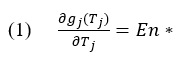
The process can be broken down into two steps. First a given time series (x_i) is shifted by its mean (see Equation 1). Then, the integrated series (X_t) is segmented by windows of different time scales (n) in which the integrated values are fit linearly per window (Y_t) and the mean squared residuals F(n) are calculated as the fluctuations of the signal (see Equation 2).

The fluctuations F(n) are a measure of variability at specific resolutions (n), that come from the averaged dispersion of residuals extracted from the local linear fits of the integrated values (X_t). Power law scaling is demonstrated through log-log plotting of F(n) over (n) in a fluctuation plot and its trend linear as delineated by the α scaling exponent which approximates the Hurst exponent. This is in reference to the original work demonstrating a heuristic measure of long-range dependence in signals dominated by stochastic properties, termed the Hurst exponent (Hurst, 1951). Newer measures such as DFA are applied to varying natural data in the attempt to estimate Hurst scaling.
The DFA method faced criticism for its ability to create artifactual curvature in the fluctuation plot. Despite its original intent to handle non-stationary noise, the robustness of the method was shown to be limited to signals with either purely stationary or weak-nonlinear trends (Bryce & Sprague, 2012). Results from the testing of artifactual curvature in DFA put many studies into question. In the case of complexity matching or the related strong anticipation studies, the strength of correlations between α scaling exponents can be problematic for unknown variability coming from artifactual curvature. Newer methods have attempted to go beyond and use a multi-fractal version of the DFA, which is further reviewed in this paper.

Allan Factor

The first use of Allan Factor for complexity matching was implemented in a dyadic task, comparing affiliative and argumentative conversations (Abney et al., 2014). Motivations to use the Allan Factor method were to bypass issues from DFA and to practically analyze rich natural data and not use the whole raw signal. As previously discussed, the DFA was shown to add artifactual curvature, which would be problematic for signals who have meaningful deviations of perfect self-similarity. A later study which looked at the HTS of various natural sounds using Allan Factor e.g., bird songs, whale song, classical music, jazz, conversations, monologues, and so on, found that certain sounds had distinct HTS. Despite jazz and conversations having obvious perceptual differences when we listen to them, Allan Factor analysis demonstrated that such two categories of sound could be grouped together as following a distinct scaling when comparing it to classical music, which was found to have similar scaling as thunderstorms along with other comparisons that broke from the norm of signals with scale-invariance (Kello, Bella, Médé, & Balasubramaniam, 2017). Many of these signals have characteristic flattening of variance and it differs across HTS groupings, therefore a method that can capture meaningful curvature in rich natural data is useful for the comparison across signal types.
For the Allan Factor to be able to normalize across scaling characteristics of signals, the method relies on an event series for its analysis of dispersion. The event series in the Abney et al., (2014) study were based on acoustic events. This is in reference to Pickering & Garrod’s (2004) interactive alignment model, in which it describes different levels of linguistic units being affected through social interaction e.g., semantic, syntactic, phonological, and phonetic, and the acoustic onsets being markers for relevant and perceivable events of acoustic energy (Cummings & Port, 1998). Future implementations of Allan Factor use peak-amplitude events due to its universality in signal processing and simplicity in identification, although events can be extracted in other ways. We stick to further explaining Allan Factor through peak-amplitude events here.
The method starts by taking a signal, often down sampled, and segmenting it into 4 min segments. For each segment the Hilbert envelope is calculated and from the produced amplitude envelope peaks are chosen in two steps. First maximal peaks are identified through a 5 ms sliding window. Then, any peaks below the H amplitude threshold are zeroed out to clean up irrelevant noise peaks occurring in low amplitude moments of the signal i.e., during a pause in speech background noise can be picked up. The H amplitude threshold is set so that one event is identified every 200 samples. Then the Allan Factor is used to take the variance at different timescales of events. At timescale T, the average of squared event differences across windows is divided by twice the mean of events across windows (see Equation 3).

This essentially gives a coefficient of variance at timescale T for what is typically done at 11 levels of resolution spanning from T ~ 30 ms to T ~ 30 s. Then results are projected in a log-log plot. The scaling of A(T) presents a power law relationship in the signal when α>0 in T^α and a flattening of such a scaling is akin to short-range correlations.

Multi Fractal

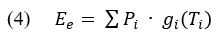
A study by Delignières et al., (2016) revisited data on bimanual and interpersonal coordination along with synchrony to a fractal metronome using multifractal detrended fluctuation analysis (MF-DFA). Motivations for the multifractal implementation were to provide a clearer picture on local adjustments versus global attunement to better define complexity matching. We have reviewed the skepticism cast on DFA due to artifactual curvature but MF-DFA use in complexity matching has not explicitly been described as a response to that. The MF-DFA starts in the same fashion as DFA (see Equations 1 & 2). Once you have the detrended fluctuations F^2 (n,s) for window segments n of size s, the next step is to average them to the qth order (see Equation 4).

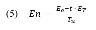
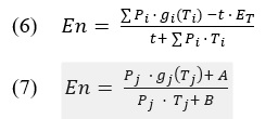
In order to get the generalized Hurst exponent h(q), a range of q values are considered and then averaged together. The q exponent cannot take a zero value, but Delignières et al., (2016) provides a logarithmic procedure (see Equation 5) as an alternative when they test q at an integer range of -15 to +15.

Also, several window sizes are used to test local adjustments versus global attunement, although one can stick to a one window size if that is not the case.

            Motivation to use MF-DFA has been to provide a clearer picture of the complexity of a time series as opposed to ‘monofractal’ methods. The metaphorical description of a ‘clearer picture’ points to monofractal methods as being limited due to only being able to capture the outline of a portrait. On the other hand, multifractality can outline subsystem details that would give more fidelity to the assumption that the picture in question is indeed of a person and not a stack of fruits. A recent paper pushed this argument, saying that assumptions of nonlinearity and within system interactions may have faith misplaced with just monofractal methods. The presented argument also did not make clear what cognitive analog multifractal cascades are responsible for capturing although it firmly called for the necessity to include multifractality (Kelty-Stephen & Wallot, 2017). Such a provocative claim explicitly explained that it could not discount monofractal methods as describing how information is embedded across scales, in the fashion to which Allan Factor has been used to measure HTS. Nevertheless, the original presentation of MF-DFA was purposed in proving its practicality for higher performance on shorter time series, which in our review we stick to as the solid consideration for such a method.  

Relating Signals

Apart from getting a measure of complexity, the process of complexity matching then needs to find a way to relate those measured complexities. An example of relating signal complexity has been used in the complexity matching literature. The cross-correlation method has been initially useful in demonstrating phase and period correction in SMS studies as a marker for synchronization (Repp, 2005; Repp & Su, 2013). Given the comparison of two signal functions f and g, the method takes their dot product (g⋆f) and correlates them at different lag points (e.g., -1, 0, and 1). The comparison between lag points allows to check how much one signal needs to be shifted in order align with another. Furthermore, one can pick a sliding window size to adjust for the resolution of cross-correlation, a window with fewer data points will compare smaller activity. The Marmelat & Delignières (2012) study adjusted windows in their cross-correlation to test local dependencies in an interpersonal coordination task. In their analysis, lag 0 correlations were meant to find simultanous event alignment and in comparison lag ±1 tested for short-range dependence between participants.
Results comparing scaling exponents and cross-correlation demonstrated a difference between the coordination of local adjustments and the matching of global activity. Researchers used such results for proof of differentiating between anticipaiton of local activity (weak anticipation) versus the anticipation that seeks to match the activity at a global scale (strong anticipation). Because cross-correlation could not fully explain the matching of scaling exponents in measured signals, the literature moved to using the term complexity matching. This is due to the theoretical predictions made by West & Grigolini (2008), in which the global activity of a signal is restricted by the complexity of the system generating it. In sum, cross-correlation was solidified to be useful in revealing local adjustments, but the complexity matching paradigmn calls for the comparison of the global scaling of a signal. Other methods have been used to provide evidence for coordination and synergies of behaviors. This includes cross-spectrum analysis which is essentially cross-correlation of the frequency domain. As well as cross recurrence analysis which measures the stability of similar activity across various embedding dimensions. Coordination literature have used such methods to provide evidence for the coupling of interpersonal and intrapersonal coordination of motor movements (Zbilut & Webber, 1992; Marwan, Wessel, Meyerfeldt, Schirdewan, & Kurths, 2002; Riley, Richardson, Schockley, & Ramenzoni, 2011). On the other hand, complexity matching uses a measure of HTS and correlates the two HTS functions. Such a correlation relates scaling instead of independent state spaces over time. The measurement of HTS retrieves a unified complexity measure across scales as opposed to sampling varying embedding dimensions. This allows one to look at the behavior as a whole and to make inferences for which timescales may be more relevant in the coupling given that scaling demonstrate how scales are related to one another in their dynamics.

Structural Resonance

So far, we have reviewed the historically relevant complexity matching studies and the methodologies involved. Empirical work has focused on interpersonal, intrapersonal, and adjustments to a chaotic metronome. From these we have seen that the work touches upon two modalities of information, movement and speech production. The procedure for finding complexity matching thus involves measuring the scaling over several timescales and correlating it to the corresponding signal from the coordinated behavior at hand. From a theoretical point of view, the production of the signals come from complex systems whose structure shape the signal. Originally modeled through complex networks (West & Grigolini, 2008), the complex structure of the networks determines how receptive they are to signals. Namely, being the most sensitive to signals with the same complex structure as the receiving network. Therefore, information is maximally transferable when communicating networks have matching complexity. Advancement in theoretical work has been interested in tackling how the brain could do complexity matching, as measured by the global cortical dynamics (Allegrini et al., 2009; Mafahim, Lambert, Zare, & Grigolini, 2015). Using data from electroencephalograph (EEG) measurements of resting states in participants, it was seen that spontaneous brain activity generated ideal 1/f signals. Ideal in this case characterized by the scaling exponent μ≈2 of renewal events. In which such events are independent and reoccurring, while still being able to characterize extended memory in a system. In connection to predictions by complexity matching theory, it is posed that the brain is most sensitive to not just 1/f, but specifically to its μ≈2 scaling. In criticality theory, μ<2 is descriptive of systems without stable extended memory while μ>2 describes an extended memory in which its stable state would take an infinite amount of time to converge from an out of equilibrium state. Many natural systems produce 1/f activity, although they may deviate from the concept of ideal event scaling. Such a pervasiveness of 1/f has led to the hypothesis of metastability. Meaning that correlated activity across multiple scales follow a homeostatic process in which ideal activity is an attractor state in the face of perturbations to the system. Furthermore, it allows for flexibility in adaptation to state changes (Kello, Anderson, Holden, & Van Orden, 2008; Kello et al., 2010). The brain then being malleable enough to attune to varying signals while also strong enough to come back to its original shape.
Empirical work demonstrating complexity matching of external stimuli and the neural oscillations has not been seen so far, or at least not directly investigated (*see addendum). There may be many reasons for why that is, including the sociology of science, lack of collaborations, debates of theoretical predictions and so on. We have reviewed how the DFA has faced criticism even when working with data less noisy than brain responses, and the argument brought forth to implement multi-fractal methods to capture clearer insights. Furthermore, EEG methods which have been typically used to capture cortical dynamics face many limitations in their experimental set up to avoid artifact production, something which behavioral experiments in the complexity matching literature do not need to worry about as much. From an empirical point of view, the biggest challenge is to control for as much cortical noise as possible if we would like to test how the structure of a stimulus can be related to a brain response. In reference to the metastability theory and complexity matching predictions, we should not expect that the brain is too easily perturbed that it will have the same extent of complexity matching that has been seen in behavioral experiments. On the other hand, it does lead us to believe that the flexibility of attunement in cortical dynamics should be sensitive enough to reflect the perceived structure of an attended stimulus. The challenge is that this becomes a needle in the haystack situation. The needle being the stimulus structure resonating in the large haystack of cortical dynamics pervasively ringing a 1/f tune.

Much of the advancement towards complexity matching theory, both theoretical and empirical, has been a relatively recent endeavor. Despite this, the idea of relating environmental complexity to brain dynamics is not as new. A relatively older study set out to explicitly match complexity from environmental stimuli to cortical dynamics (Tononi, Sporns, & Edelman, 1996). They used a cortical vision neural network model instead of directly measuring brain responses and their stimuli were a set of elongated vertical or horizontal bars. They compared the visual model to a randomly connected version of the model and measured the entropy of the stimulus and model activity. The matching was done by taking a difference between stimulus and model entropy, and results showed that the random connectivity in the model had a significantly bigger difference than the relevant functional connectivity. Empirical work has made advancements in methodology to relate complex natural stimuli and brain response. A study by Lalor & Foxe (2010) developed what is termed as Auditory Evoked Spread Spectrum Analysis to have a brain response using EEG with high temporal resolution. As it relates to our purposes of complexity matching, the limitations to this technique is that it requires an averaging over multiple presentation blocks, ~48 mins in their study. It also is stimulus driven by requiring the use of the stimulus amplitude to do least squares estimation on the response, as well as responses being akin to Event Related Potentials which do not directly reflect the complex structure of the signals. In another case, Skoe & Kraus (2010) describe a method for finding neural synchrony to auditory stimuli using complex Auditory Brainstem Responses (cABR). Stimuli take a short clip of any complex auditory stimuli, typically no more than 10 seconds long, and present it ~2000-3000 times. The collected cABRs have high temporal and spectral resolution which holds enough information to reconstruct the signal and play it back, sounding very similar to the original stimulus. Furthermore, the use of natural speech stimuli presented at isochronous intervals have been used to demonstrate hierarchical cortical tracking of semantic units (Ding, Melloni, Zhang, Tian, & Poeppel, 2015). Neural responses show tracking occurring at the sentence level (1Hz), phrase level (2Hz), and syllable level presented as monosyllabic morphemes (4Hz). Similarly, evidence for a hierarchical system in auditory processing is posited by demonstrating tracking at lower frequencies of phonemic units in natural speech ~155s (Di Liberto, O’Sullivan, & Lalor, 2015). Longer stimuli are also used in the attempt to analyze hierarchical processing of music and speech with lengths closer to their natural lengths ~4:15 mins (Farbood, Heeger, Marcus, Hasson, & Lerner, 2015). They present conditions with scrambled structure at three different timescales of the music separately to trained musicians. Using fMRI, larger musical timescales were found to be processed longer when approaching higher order brain topography in the auditory cortex.

As presented above, there has been much work trying to develop methods and testable hypothesis to understand how complexity of stimuli such as speech and music can be explained to resonate in cortical dynamics. The idea of complexity matching of complex natural stimuli such as music and speech with brain responses is just one of the testable hypotheses in this space of work. The development of a method that can show substantial evidence for complexity matching will have a large impact even outside the complexity matching theory. The problem of the needle in the haystack is what stands in the way. In order to approach this problem, there seems to be two routes to take. One is to put effort into enhancing the hidden signal per stochastic resonance approaches or to use a stimulus driven approach in the extraction of the signal to enhance impoverished features. This type of approach may be informative and present unique testable hypotheses for how to think of complexity matching in brain responses, but it also may be perceived as a less faithful approach to the question at hand. Second is to control for cortical noise as much as possible, in other words, to make the hay as small as possible. This direction is preferable in order to more faithfully compare the strength of structural resonance in cortical dynamics. Careful artifact filtering and pre-processing should be paid attention to because it may not be as obvious as to what in the signal can be considered as noise. We predict that non-stationarities in cortical dynamics may be harder to deal with and thus affect the visibility of structural resonance. A recently more popular method in analyzing complexity in EEG time series is multiscale entropy (MSE). A study reviewed guidelines for the interpretation of MSE on EEG (Courtiol et al., 2016). Such a method of analysis allows for capturing both linear and nonlinear autocorrelations but with the resolution of complexity focusing in the shorter timescales. There has not been a study addressing an explicit finding on a nonlinear autocorrelation for complexity matching, although the literature always assumes that the signals are generated through a nonlinear function. Although scaling functions correlated to check for complexity matching may present nonlinear scaling, the studies have found it sufficient to correlate linear fits. We consider the exploration of MSE to be worth taking in complexity matching endeavors to brain responses, even if all it is doing is giving us a more detailed picture of the aggregate trends. Furthermore, we expect that it would be beneficial to work with an event series as opposed to raw signals of complex auditory stimuli and EEG. Both due to the practical computation, and abstraction of meaningful variation used to bypass expected non-stationaries. The AF method has proven itself to be reliable in several studies involving complex natural stimuli, although there seems to a stronger representation of the longer timescales. This could be mitigated when combined with MSE who is sensitive to activity in smaller timescales.

Discussion

Complexity matching has been used in empirical studies to quantify coordination. In the abstract, the complexity matching theory describes that maximal information transfer between complex networks occurs when they have their structures scale the same way. From an empirical point of view, participants are put into scenarios in which they produce signals in correspondence to a coupled behavior with another participant. Those signals then have their scaling over multiple timescales measured and the scaling exponent of both signals are correlated. The HTS of a signal is said to be non-trivially matched in a dyadic task. Both participants make an effort in how they produce those signals to have a matching. This happens through a combination of local adjustments and global attunement. In the example of coordinating language, we can refer back to the interactive alignment model (Pickering & Garrod, 2004). The model can be summarized as demonstrating two things: the importance of the embedded relationship of linguistic units, and that alignment can happen at various levels of linguistic units. An extreme example of coupling can be through finding synchrony. If two interlocutors can produce continuous speech at the same time with the same information contained, then it becomes a clear indication of coupling. Such an example is exemplary of a parlor trick, but it denotes a perceivably distinct case in which an observer can tell that two individuals are coupled. On the other hand, coordination may be harder to observe in a conversation because it is not obvious how my speech production is aiding the other’s. With the assumption that both speakers want to listen and process as much of each other’s speech signals as possible, speakers will attempt to converge on the same signal ‘frequency’ much like communication between two walkie-talkies. Whether most people can directly influence fast timescales akin to sub-syllabic units is an untested hypothesis. On the other hand, complexity matching in language has shown that the main coupling relation is housed at the longer timescales (Schneider et al., 2019). Studies using Allan Factor analysis to get a scaling function of speech have attributed their measurements as quantifying prosody (Falk & Kello, 2017). It has also been shown that manipulating speaking rate has an effect on HTS of speech (Ramirez-Aristizabal et al., 2018). Which raises another testable hypothesis for whether the longer timescales can be said to facilitate the embedding of smaller linguistic units and thus shaping the alignment of interlocutors.
A recent study has taken complexity matching methods to inform physical therapy for locomotion. They had young and elderly participants, in which the young participants produced a healthy 1/f scaling of their stride durations and the older participants produced signals more akin to white noise, reflecting a drop in complexity (Almurad, Roume, Blain, & Delignières, 2018). The elderly participants showed a two-week sustained correction of their locomotion after walking hand in hand with a young participant for three weeks. Such a therapeutic endeavor to implement complexity matching allowed for interesting testable hypotheses to arise. One of them putting forth the question whether it makes sense to think of a pervasive 1/f signal generator as an attractor to signals that deviate from that. More generally, it also prompts the hypothesis that a signal with ‘more’ complexity can pull a ‘less’ complex signal. Such findings are informative for therapeutic engineering applications beyond locomotion such as virtual agent/chat bot counseling in the mental healthcare space. The movement of counseling and therapy to happen in an online space is meant to increase accessibility for patients who otherwise would find it difficult to physically reach out to their health care providers or live in areas with poor healthcare infrastructure (D’Alfonso et al., 2017; Tielman, Neerincx, Bidarra, Kybartas, & Brinkman, 2017). Complexity matching methods can be applied to understanding the prosody of depression. A study tackling such an issue analyzed counseling sessions of depressed patients and their therapists. One of their analyses focused on the speech produced and found that when comparing the prosody of the counselor to the patient, less depressed patients had similar prosodic features to their therapists (Yang, Fairbairn, & Cohn, 2013). Prosodic features included the fundamental frequency of a speaker and the lag time between the utterance of one speaker to the other (switching pause). The results showed that the therapists had a significantly higher variability in their fundamental frequency compared to the depressed patients and that switching pause was shorter for less depressed patients. These results converge with the idea that turn taking and variability of linguistic units being what underlies complexity matching in speech (Abney et al., 2014; Schneider et al., 2019). Furthermore, prosodic embellishment has been shown to produce HTS that is more complex (Falk & Kello, 2017) and less natural speech has less complexity (Ramirez-Aristizabal et al., 2018).
These hypotheses of regulating complexity through the coupling of a stronger, pervasive 1/f signal can be informative when thinking about complexity matching with brain responses. We know that the brain produces global 1/f cortical dynamics, and that theory predicts that sensibility is strongest for signals akin to it. We also know that the brain is flexible and that the productions of 1/f can be a sign of metastability. This would allow for the combination of sturdiness to a 1/f stable state and sensitivity to attune to varying signals. These theoretical predictions do not say much in terms of how to test for complexity matching with neural oscillations. What it does help in is thinking about complexity matching in the brain as a search for a change in affect from its steady state, or how the structural resonance of stimuli can be captured. This is very similar to the case of doing complexity matching between a person and a chaotic metronome. An example of such an implementation would be to measure the awake resting state of a participant and compare it to the entrainment of a complex signal to see whether the stable state of spontaneous 1/f production can be affected. This implementation requires multiple averaged presentations of a complex stimuli and the length of the presentations would need to be representative of the HTS of the signal, which in the case of natural stimuli such as speech and music would require it to be in the order of minutes. This complicates the length of an entrainment session and makes it harder to keep a participant focused on the task, which will increase the chance of cortical noise. In the case of trying to test whether healthy state neural oscillations can attract weaker, whitened cortical dynamics, one could measure the EEG responses of coupled individuals in a task. This would need the capability to bypass muscle artifacts to which social interactions often require. To remedy this, a virtual reality study could be adapted so that virtual interactions help control for the need of physical exertion (Zapata-Fonseca et al., 2016). We conclude by making the point that complexity matching in the brain requires careful consideration for artifacts in the data because the slightest perturbation is reflected in our cortical dynamics. Despite that, we believe that we can find the corresponding reflection pool to our auditory world.

Addendum

A study tackling many of the issues brought up in this review has been published after the review was written. The study focused on how the correlated structure of music stimuli and the corresponding EEG response can be an index for mediating music listening pleasure (Borges et al., 2019). In brief the experiment had 12 classical music presentations (~2 min length) while participants closed their eyes and they were rated on their listening pleasure after. Although the study did not explicitly make their narrative about complexity matching, we believe that their data do put forth the first example of complexity matching with EEG responses in the literature so far. They did use DFA and correlated slopes of only classical music which as previously mentioned in this paper follows a 1/f scaling structure. This review has shown that there may be some issues with only using DFA and that there is strong theoretical grounding on structural resonance especially at the scaling that approximates the ideal 1/f statistics. However, current endeavors in our personal research at the Cognitive Mechanics lab and our affiliated collaborators have taken this study with great confidence to then propose a study focused solely on establishing complexity matching theory with EEG responses using their methodology for data cleaning and experimental set up. The hope is that their success in using PREP pipeline and Empirical Mode Decomposition to clean and separate the signal without worrying about artifacts can be transferred into an experimental paradigm that tests a variety of complex acoustic signals to see that limits of matching. Putting forth a scientific study that stakes the theoretical claim of complexity matching brings about more theoretical baggage about the information transfer between systems and can open up avenues for testing the theoretical predictions that we have mentioned above.

References

Abney, D. H., Paxton, A., Dale, R., & Kello, C. T. (2014). Complexity matching in dyadic conversation. Journal of Experimental Psychology: General. Abney, Drew H.: Cognitive and Information Sciences, University of California, Merced, School of Social Sciences, Humanities and Arts, 5200 North Lake Road, Merced, CA, US, 95343, drewabney@gmail.com: American Psychological Association. https://doi.org/10.1037/xge0000021

Allegrini, P., Menicucci, D., Bedini, R., Fronzoni, L., Gemignani, A., Grigolini, P., … Paradisi, P. (2009). Spontaneous brain activity as a source of ideal 1/f noise. Physical Review E – Statistical, Nonlinear, and Soft Matter Physics, 80(6), 1–13. https://doi.org/10.1103/PhysRevE.80.061914

Almurad, Z. M. H., Roume, C., Blain, H., & Delignières, D. (2018). Complexity Matching: Restoring the Complexity of Locomotion in Older People Through Arm-in-Arm Walking   . Frontiers in Physiology  . Retrieved from https://www.frontiersin.org/article/10.3389/fphys.2018.01766

Almurad, Z. M. H., Roume, C., & Delignières, D. (2017). Complexity matching in side-by-side walking. Human Movement Science, 54, 125–136. https://doi.org/https://doi.org/10.1016/j.humov.2017.04.008

Baronchelli, A., Ferrer-i-Cancho, R., Pastor-Satorras, R., Chater, N., & Christiansen, M. H. (2013). Networks in Cognitive Science, 17(7), 348–360. https://doi.org/10.1016/j.tics.2013.04.010

Borges, A. F. T., Irrmischer, M., Brockmeier, T., Smit, D. J., Mansvelder, H. D., & Linkenkaer-Hansen, K. (2019). Scaling behaviour in music and cortical dynamics interplay to mediate music listening pleasure. Scientific reports9(1), 1-15.

Bryce, R. M., & Sprague, K. B. (2012). Revisiting detrended fluctuation analysis. Scientific Reports, 2, 315. Retrieved from https://doi.org/10.1038/srep00315

Coey, C. A., Washburn, A., Hassebrock, J., & Richardson, M. J. (2016). Complexity matching effects in bimanual and interpersonal syncopated finger tapping. Neuroscience Letters, 616, 204–210. https://doi.org/10.1016/j.neulet.2016.01.066

Courtiol, J., Perdikis, D., Petkoski, S., Müller, V., Huys, R., Sleimen-Malkoun, R., & Jirsa, V. K. (2016). The multiscale entropy: Guidelines for use and interpretation in brain signal analysis. Journal of Neuroscience Methods, 273, 175–190. https://doi.org/https://doi.org/10.1016/j.jneumeth.2016.09.004

Cummings, F., & Port, R. (1998). Rhythmic constraints on stress timing in English. Journal of
            Phonetics
26, 145-171.

D’Alfonso, S., Santesteban-Echarri, O., Rice, S., Wadley, G., Lederman, R., Miles, C., … Alvarez-Jimenez, M. (2017). Artificial Intelligence-Assisted Online Social Therapy for Youth Mental Health   . Frontiers in Psychology  . Retrieved from https://www.frontiersin.org/article/10.3389/fpsyg.2017.00796

Dale, R., Fusaroli, R., Duran, N. D., & Richardson, D. C. (2013). Chapter Two – The Self-Organization of Human Interaction. In B. H. B. T.-P. of L. and M. Ross (Ed.) (Vol. 59, pp. 43–95). Academic Press. https://doi.org/https://doi.org/10.1016/B978-0-12-407187-2.00002-2

Delignières, D., Almurad, Z. M. H., Roume, C., & Marmelat, V. (2016). Multifractal signatures of complexity matching. Experimental Brain Research, 234(10), 2773–2785. https://doi.org/10.1007/s00221-016-4679-4

Dubois, D. M. (2003). Mathematical Foundations of Discrete and Functional Systems with Strong and Weak Anticipations BT  – Anticipatory Behavior in Adaptive Learning Systems: Foundations, Theories, and Systems. In M. V Butz, O. Sigaud, & P. Gérard (Eds.) (pp. 110–132). Berlin, Heidelberg: Springer Berlin Heidelberg. https://doi.org/10.1007/978-3-540-45002-3_7

Falk, S., & Kello, C. T. (2017). Hierarchical organization in the temporal structure of infant-direct speech and song. Cognition, 163, 80–86. https://doi.org/https://doi.org/10.1016/j.cognition.2017.02.017

Fine, J. M., Likens, A. D., Amazeen, E. L., & Amazeen, P. G. (2015). Emergent complexity matching in interpersonal coordination: Local dynamics and global variability. Journal of Experimental Psychology: Human Perception and Performance. Fine, Justin M.: Department of Psychology, Arizona State University, Box 871104, Tempe, AZ, US, 85287, justin.fine@asu.edu: American Psychological Association. https://doi.org/10.1037/xhp0000046

Freeman, W. J. (2005). A field-theoretic approach to understanding scale-free neocortical dynamics. Biological Cybernetics, 92(6), 350–359. https://doi.org/10.1007/s00422-005-0563-1

Gan, L., Huang, Y., Zhou, L., Qian, C., & Wu, X. (2015). Synchronization to a bouncing ball with a realistic motion trajectory. Scientific Reports, 5, 11974. Retrieved from https://doi.org/10.1038/srep11974

Grigolini, P., Aquino, G., Bologna, M., Luković, M., & West, B. J. (2009). A theory of 1/f noise in human cognition. Physica A: Statistical Mechanics and Its Applications, 388(19), 4192–4204. https://doi.org/https://doi.org/10.1016/j.physa.2009.06.024

Hofstadter, D. R. (1979). Gödel, Escher, Bach: an eternal golden braid (Vol. 20). New York:
            Basic books.

Hove, M. J., Iversen, J. R., Zhang, A., & Repp, B. H. (2013). Synchronization with competing visual and auditory rhythms: bouncing ball meets metronome. Psychological Research, 77(4), 388–398. https://doi.org/10.1007/s00426-012-0441-0

Iversen, John R, Patel, A. D., Nicodemus, B., & Emmorey, K. (2015). Synchronization to auditory and visual rhythms in hearing and deaf individuals. Cognition, 134, 232–244. https://doi.org/https://doi.org/10.1016/j.cognition.2014.10.018

Iversen, John Rehner, & Balasubramaniam, R. (2016). Synchronization and temporal processing. Current Opinion in Behavioral Sciences, 8, 175–180. https://doi.org/https://doi.org/10.1016/j.cobeha.2016.02.027

Kello, C. T., Anderson, G. G., Holden, J. G., & Van Orden, G. C. (2008). The Pervasiveness of 1/f Scaling in Speech Reflects the Metastable Basis of Cognition. Cognitive Science, 32(7), 1217–1231. https://doi.org/10.1080/03640210801944898

Kello, C. T., Brown, G. D. A., Ferrer-i-Cancho, R., Holden, J. G., Linkenkaer-Hansen, K., Rhodes, T., & Van Orden, G. C. (2010). Scaling laws in cognitive sciences. Trends in Cognitive Sciences, 14(5), 223–232. https://doi.org/https://doi.org/10.1016/j.tics.2010.02.005

Kelty-Stephen, D. G., & Wallot, S. (2017). Multifractality Versus (Mono-) Fractality as Evidence of Nonlinear Interactions Across Timescales: Disentangling the Belief in Nonlinearity From the Diagnosis of Nonlinearity in Empirical Data. Ecological Psychology, 29(4), 259–299. https://doi.org/10.1080/10407413.2017.1368355

Lalor, E. C., & Foxe, J. J. (2010). Neural responses to uninterrupted natural speech can be extracted with precise temporal resolution. European Journal of Neuroscience, 31(1), 189–193. https://doi.org/10.1111/j.1460-9568.2009.07055.x

Mafahim, J. U., Lambert, D., Zare, M., & Grigolini, P. (2015). Complexity matching in neural networks. New Journal of Physics, 17(1), 15003. https://doi.org/10.1088/1367-2630/17/1/015003

Marmelat, V., & Delignières, D. (2012). Strong anticipation: complexity matching in interpersonal coordination. Experimental Brain Research, 222(1), 137–148. https://doi.org/10.1007/s00221-012-3202-9

Marwan, N., Wessel, N., Meyerfeldt, U., Schirdewan, A., & Kurths, J. (2002). Recurrence-plot-based measures of complexity and their application to heart-rate-variability data. Physical review E66(2), 026702.

McAuley, J. D., & Henry, M. J. (2010). Modality effects in rhythm processing: Auditory encoding of visual rhythms is neither obligatory nor automatic. Attention, Perception, & Psychophysics, 72(5), 1377–1389. https://doi.org/10.3758/APP.72.5.1377

Patel, A. D. (2003). Language, music, syntax and the brain. Nature neuroscience6(7), 674.

Patel, A. D., & Iversen, J. R. (2014). The evolutionary neuroscience of musical beat perception: the Action Simulation for Auditory Prediction (ASAP) hypothesis   . Frontiers in Systems Neuroscience  . Retrieved from https://www.frontiersin.org/article/10.3389/fnsys.2014.00057

Patel, A. D., Iversen, J. R., Chen, Y., & Repp, B. H. (2005). The influence of metricality and modality on synchronization with a beat. Experimental Brain Research, 163(2), 226–238. https://doi.org/10.1007/s00221-004-2159-8

Peng, C.-K., Buldyrev, S. V, Havlin, S., Simons, M., Stanley, H. E., & Goldberger, A. L. (1994). Mosaic organization of DNA nucleotides. Physical Review E, 49(2), 1685–1689. https://doi.org/10.1103/PhysRevE.49.1685

Pickering, M. J., & Garrod, S. (2004). Toward a mechanistic psychology of dialogue. Behavioral and Brain Sciences, 27(2), 169–190. https://doi.org/DOI: 10.1017/S0140525X04000056

Riley, M. A., Richardson, M., Shockley, K., & Ramenzoni, V. C. (2011). Interpersonal synergies. Frontiers in psychology2, 38.

Ramirez-Aristizabal, A. G., Médé, B., & Kello, C. T. (2018). Complexity matching in speech: Effects of speaking rate and naturalness. Chaos, Solitons & Fractals, 111, 175–179. https://doi.org/10.1016/j.chaos.2018.04.021

Repp, B. H. (2005). Sensorimotor synchronization: A review of the tapping literature. Psychonomic Bulletin & Review, 12(6), 969–992. https://doi.org/10.3758/BF03206433

Repp, B. H., & Su, Y.-H. (2013). Sensorimotor synchronization: A review of recent research (2006–2012). Psychonomic Bulletin & Review, 20(3), 403–452. https://doi.org/10.3758/s13423-012-0371-2

Skoe, E., & Kraus, N. (2010). Auditory brainstem reponse to complex sounds : a tutorial. Ear Hear, 31(3), 302–324. https://doi.org/10.1097/AUD.0b013e3181cdb272.Auditory

Stephen, D. G., Stepp, N., Dixon, J. A., & Turvey, M. T. (2008). Strong anticipation: Sensitivity to long-range correlations in synchronization behavior. Physica A: Statistical Mechanics and Its Applications, 387(21), 5271–5278. https://doi.org/https://doi.org/10.1016/j.physa.2008.05.015

Stepp, N., & Turvey, M. T. (2010). On Strong Anticipation. Cognitive Systems Research, 11(2), 148–164. https://doi.org/10.1016/j.cogsys.2009.03.003

T., K. C., Dalla, B. S., Butovens, M., & Ramesh, B. (2017). Hierarchical temporal structure in music, speech and animal vocalizations: jazz is like a conversation, humpbacks sing like hermit thrushes. Journal of The Royal Society Interface, 14(135), 20170231. https://doi.org/10.1098/rsif.2017.0231

Tielman, M. L., Neerincx, M. A., Bidarra, R., Kybartas, B., & Brinkman, W.-P. (2017). A Therapy System for Post-Traumatic Stress Disorder Using a Virtual Agent and Virtual Storytelling to Reconstruct Traumatic Memories. Journal of Medical Systems, 41(8), 125. https://doi.org/10.1007/s10916-017-0771-y

Tononi, G., Sporns, O., & Edelman, G. M. (1996). A complexity measure for selective matching of signals by the brain. Proceedings of the National Academy of Sciences, 93(8), 3422 LP – 3427. https://doi.org/10.1073/pnas.93.8.3422

West, B. J., Geneston, E. L., & Grigolini, P. (2008). Maximizing information exchange between complex networks. Physics Reports, 468(1–3), 1–99. https://doi.org/10.1016/j.physrep.2008.06.003

Yang, Y., Fairbairn, C., & Cohn, J. F. (2013). Detecting Depression Severity from Vocal Prosody. IEEE Transactions on Affective Computing, 4(2), 142–150. https://doi.org/10.1109/T-AFFC.2012.38

Zapata-Fonseca, L., Dotov, D., Fossion, R., & Froese, T. (2016). Time-Series Analysis of Embodied Interaction: Movement Variability and Complexity Matching As Dyadic Properties   . Frontiers in Psychology  . Retrieved from https://www.frontiersin.org/article/10.3389/fpsyg.2016.01940 Zbilut, J. P., & Webber Jr, C. L. (1992). Embeddings and delays as derived from quantification of recurrence plots. Physics letters A171(3-4), 199-203.

Optimal Foraging Theory: Foraging in the Face of Uncertainty

Abstract

Classic Optimal Foraging Theory (OFT) originally outlined food finding behavior through the Marginal Value Theorem (MVT), which describes the best time to move onto a new resource patch. The extension of the MVT to cognitive processes has allowed for the testing beyond the ideal observed behavior and into mechanistic processes that give rise to foraging behavior. At the core of the theory is the definition of the Optimal Forager, which place the assumptions necessary to describe the generalizability of the MVT. The original Optimal Forager definition held an orientation towards a behaviorist epistemology which allowed for high generalizability of the behavior. On the other hand, testing foraging as a cognitive process allowed researchers to ask questions beyond the ideal Optimal Forager definition and focus on variability in habitats as well as uncertainties foragers face in relevance to internal mechanistic processes. In this paper we will review canonical OFT and how it has been expanded into cognitive processes. We will also break down the assumptions that make the model work and in which cases those assumptions are limited. An argument is presented for defining a Heuristic Forager, which is used to formally update foraging epistemology trends in cognitive oriented research that was not set in the original Optimal Forager definition.

Intro

The problem of search shows itself across disciplines and varies widely in model implementations. Researchers have pointed out that search processes are behaviors that can generalize across species and types of habitats. On one hand, search behavior can be seen in plant roots trying to localize water, bacteria seeking nutrients, birds hunting for fish in the ocean, or early humans searching for edible berries in bushes (Koshland 1980; Weimerskirch, Salamolard, Sarrazin, & Jouventin, 1993; Eisenbach & Lengeler 2004; Raichlen et al., 2014). On the other hand, search behavior can also be seen when looking for a mate, searching your memory for a specific word, looking for hotel prices online, or when babies look for parental feedback through their babbling (Hills, Jones, & Todd, 2012; P. Pirolli & Card, 1999; Prokopy & Roitberg, 1984; Tamis-LeMonda, Kuchirko, & Song, 2014). The former presents classic cases in the behavioral ecology literature that can be framed as food finding behavior, where the goal of the search is to replenish energy to the searcher. The latter provides examples in which instead of energy consumption, the currency of trade in the search process is time. The principles of search behavior in the classic examples have been able to generalize beyond food finding behavior despite the differences in habitat, currency, and goal. This has been seen across varying types of search processes, but this paper will focus on the act of foraging. Broadly speaking, foraging involves a searcher exploring a space in order to exploit resources. When considering a balance of currency, whether it is time or energy, resources are modeled to be clustered in resource patches. This is referred to as patch foraging (Hills & Dukas, 2012). The problem of a forager in patch foraging is to determine the best way to allocate its currency as it travels from patch to patch. The two state (exploration & exploitation) switch cost balancing problem falls under the category of Optimal Control Problems. Problem sets in this category are assumed to have guidelines in which a best (optimal) solution is attainable (Kirk, 2012). In this paper we review the canonical theoretical framework for patch foraging and its model implantation for describing it as a type of Optimal Control Problem. We then demonstrate limitations to its categorization as an Optimal Control Problem by breaking down the assumptions necessary for the original model implementation. This paper concludes by providing an updated way of talking about the extension of foraging in cognitive processes.

OFT

The traditional Optimal Foraging Theory (OFT) was initially grounded in animal food finding behavior. It framed a scenario in which the food was found in patches of different magnitudes, and the predator would exhaust the resources found per patch during the search process. Varying magnitudes of patch types can include variability of reward gains per resource found and size of patch (Charnov, 1976). One can think of a classic example such as foraging for berries and the berry bushes being the resource patch. The varying sizes of bushes become indicators of how many berries a forager can extract along with varying quality of berries in that bush independent of bush size (Krebs, Kacelnik, Taylor, 1978; Pyke, 1984). For example, a forager can encounter a large bush with many berries and with berries that are at the peak ripeness to replenish maximum nutritional value per berry consumed. On the other hand, a forager can also encounter a small bush with berries that are of poor quality, meaning that the amount of nutritional value or quality of energy gained per consumption of berry is low. In an environment of depleting resources and limited energy, the problem of foraging is centered around when the best time to move onto a new resource patch is, as to not have a detrimental rate of energy intake per foraging bout (Pyke, Pulliam, & Charnov, 1977).

For a predator to be optimal in its foraging it needs to balance its energy intake over the time spent in a patch. Depleting resources will make it so that the time between successive consumption increases over time. Going back to the berry bush example, one can imagine foraging in a large berry bush and being pleased at the number of berries easily available to you. At some point, finding the rest of the berries in the bush will become more labor intensive and you will be putting too much energy into trying to fully deplete that resource patch. If a forager stays too long in a patch, then the energy intake rate will be too low for the amount of energy spent. The optimization of this behavior is therefore outlined by the Marginal Value Theorem, which states that energy intake (g_j (T_j)) over time spent in a patch (T_j) is equal to the average capture rate in the habitat (En*).

This is optimal under several more assumptions, which include a constant between patch travel cost and random encounter of patch types. This means that the length of time of traveling between patches should be independent of time spent in a patch, but the time spent in a patch will depend on the time traveling between patches. The original model holds that parameter constant to highlight time allocation in a patch without complicating the model to need to explain a rational choice analysis when traveling to different patch types (Pyke, 1984). This simplification allows the theory to focus on what an optimal forager is and how their behaviors are demonstrated to be optimal on average. Natural selection is used to explain how optimal foragers are formed to follow optimal behavior as outlined by the MVT. The caveat to this is that foragers have access to the complete information of their habitats in order to make the model work (Kamil & Yoerg, 1982; Waddington, 1985). The limitations to this definition are discussed further in the paper but for now we review the original assumptions of the model and theory.

A further breakdown of the model is needed to fully understand the theoretical bounds and epistemic purpose of using the MVT to describe optimal foraging behavior. The first parameter in the model (P_i) takes into account the proportion of the visited patches that are of type i. As previously mentioned, types of patches in this context can vary the amount of resources contained along with the type of quality of resources the patch holds. The second parameter (E_T) is used to set the energy cost of traveling between patches per unit time. The theory holds this value constant. Third, the parameter (E_si) determines how much energy to charge in a patch of type i per unit time. Given these fundamental parameters, it is possible to define how the relationships in the model are built. The gained energy from foraging for any given number of time units (T) in a patch type of i minus all energy costs that do not include the cost of foraging in a patch is denoted as h_i (T). When correcting for the energy cost of searching in a patch, the function is denoted as:

Next, the relationship that describes the average time spent in a patch (T_u) includes the time it takes to travel between patches t plus the time spent in patches.

Again, the variability of values that can come from different patch types is denoted by i and similarly it can be shown how the average energy from a patch (E_e) is described.

Given the description above, we can now present the relationship of the net energy intake rate (E_n).

Equation (5) is fundamentally an energy balancing function and with the equations presented above it becomes clear how the model acquires the values now needed to make a case for optimal behavior.

The time spent traveling between patches t is argued to be independent of the time spent in any one patch T_i , but the time spent in any one patch cannot be said to be independent of the time spent traveling between patches. For example, a forager can spend a large amount of time traveling between berry bushes but once it arrives to the bush, factors such as patch size and resource quality will determine how long a forager stays (McNamara & Houston, 1985). On the other hand, if a forager stays either too long or short in one patch, the decision to travel more or less between patches now becomes important for its survival. If an animal spends too much energy in one bush, then it will need to replenish its energy as soon as possible and a long between patch travel time would not be the most attractive choice. Given this theoretical grounding, the parameters for how to obtain the values of importance can now be compared to set what is optimal in the theory. Equation (5) is written in form (6) to equate with (7) which is now an equation that allows us to look at the process from a single patch (j) perspective.

Values A & B are the result of equating 6 & 7 and are not functions of  in which the MVT states that a forager only has control over  when patch  is visited. Finally, for all  given that all  are at their optimal values,  is written as . We then are able to describe it as equation (1), where the  average capture rate in the habitat is the optimal threshold for when to leave any patch  (Charnov, 1976).

The original model as described above faced some limitations when trying to account for the complete information an optimal forager may lack and variability of patch quality. High variability across patches makes it difficult for a forager to follow a generalized optimal policy if encounters are random and resources non-renewable. Furthermore, behavioral ecologists have not been able to mend the problem of incomplete information in food-finding behavior despite attempts to model patch sampling as a means for describing information gathering (Stephens & Krebs, 1986). Markov chain models have been used to describe patch sampling, in which an optimal forager who faces uncertainty surveys patch quality (Bobisud & Potraz, 1976; Stephens, Charnov, 1982). Modeling an optimal forager with incomplete information of their habitat has shown that it is optimal to stay longer in a patch past the optimal policy (Oaten, 1977; Green, 1980). Staying longer allows the forager to learn valuable information about their habitat such as patch type distributions and variability of reward gains (Pyke, 1984). The limitations of the original optimal forager with complete information is reviewed with the extension to cognitive processes in the next sections.

OFT in Cognition

Since the implementation of the MVT to concisely describe optimal foraging in food finding behavior, proponents of OFT have extended how the model can describe cognitive processes framed as foraging. This review highlights relevant historic publications and will not serve as an extensive list of all instances of MVT application in human cognition. One of the first examples was with the declaration of treating information spaces and their human-computer interactions as a foraging process (Pirolli & Card, 1995). Information Foraging (IF) then became the study of the trade offs that people consider in information seeking tasks, such as trying to balance the quality of information gain versus the cost of performing an activity in interaction with the design of the information space. Furthermore, the design of the information space was more commonly treated as an aid in not just the storage and handling of the information but also with the optimization of its access. Examples of this in the IF theory tested spaces anywhere from rank order search results from search engines, citation links in papers, and electronic mail to more physically tangible spaces such as office workspaces. The theory also states that human computer interaction adds another dimension to information foraging. That is to say that people put in effort to enrich the foraging process because of the ability to design information spaces (Pirolli & Card, 1999).

A key distinction from the classic food finding forager in IF is the ability for a forager to design their information spaces which involves a focus on rational thought. For our purposes, rational thought is used in connection to the ability to design and enrich our information spaces for the purposes of optimizing the gains of foraging behavior. Something that an optimal forager from a behaviorist perspective can offload to natural selection and not to internal cognitive processes without having to worry about modeling decision making. IF theory puts its own model of higher-level cognition (ACT-IF), inspired by Anderson (1996) and the Adaptive Control of Thought – Rational (ACT-R) model for higher level cognition as a computational production system. Wayfinding and general knowledge in information spaces are described by scent detection processes, while the tradeoff dilemma of maximizing gains in current information patches is implemented by the MVT. On top of these processes, the relationship of an information forager who is capable of habitat design and purposeful foraging enrichment is explained by the ACT-IF model. A further break down of the ACT-IF model can be seen in Pirolli & Card (1999). In this section we focus on the extension of MVT implementation when framed for cognitive processes.

A more direct connection to behavioral ecology and foraging in humans came about with the testing of adaptability in foraging strategies. In reference to the classic OFT food finding behavior, an animal is adapted to their specific habitat and the knowledge needed to perform optimally over time is grounded in natural selection (Charnov, 1976; Pyke et al., 1977). The original theory did not present a description of foraging as a cognitive process but rather focused on the generalization of the behavior. Whether an animal had to make a rational choice or care about adapting its strategy to fit unknown habitats was not the original motivation for OFT. In the case of studying humans as an expert generalist, the question of adaptability in strategies became relevant in the connection to the behavioral ecology literature. Hutchinson, Wilke & Todd (2008) tackled this issue by placing participants in a fishing computer game. In the game, participants were given up to 45 mins to catch as many fish as they could and were monetarily incentivized to catch more fish. A resource patch in the game was implemented as a pond and the participant was allowed to switch to a new pond at any time without being able to run out of ponds to switch to. The conditions in the experiment varied fish across ponds from even, Poisson, and aggregated distributions. A second version of the aggregated condition made between patch travel time longer from 15 secs to 25 secs. The optimal policy for when to switch to a new patch across varying distributions is only dependent on the number of items caught in a patch N and the time spent in a patch T (Iwasa, Higashi, & Yamamura, 1981).

Theoretical predictions for optimal policies were tested through simulations to compare how participants differ from optimal. If a resource distribution is set to even, then the optimal policy is a ‘fixed-N-rule’, in which participants should leave to a new patch after finding a certain number of items. A Poisson distribution across patches has a ‘fixed-T-rule’, describing that a forager needs switch at a fixed time. In an aggregated distribution the optimal policy should be defined by the ‘incremental rule’, in which a forager extends the time in a patch for every new item found. Conversely, if the distribution is sparse then the forager should follow a ‘decremental rule’ and decrease the amount of time in a patch for every item found. The human data collected showed that people did not follow the optimal policies across conditions. Furthermore, a performance comparison with a ‘giving-up time’ heuristic was done to compare human performance with a general heuristic. In this comparison, the performance was closer than the optimal policy but still statistically different. For all conditions, people demonstrated linear positive correlations for time spent per item found in a patch. A Cox Proportional Hazards Regression model was used to determine that time between item captures was the biggest predictor for switching to a new patch. It was concluded that equating sufficient knowledge in the environment of the game was not easy and that participants were only basing their decisions from the success of their last two captures. The MVT uses the optimal forager theory to explain the robust knowledge a forager has from an environment that they developed in, which participants did not have. Therefore, a possible explanation for the data is that participants were defaulting to a heuristic as a fail-safe on their performance instead of risking the confirmation of an optimal policy.

Following the previous study’s lead, a new study sought to measure internal word search with given sequences of letters as the resource patch. A group of German speakers were given predefined letter sequences and told to create as many words as they can with that sequence, much like a game of Scrabble. Participants were monetarily incentivized to create more words and could switch to a new ‘patch’ of letter sequences whenever they deemed necessary but the movement to the next patch had a time cost. The study had limitations for defining specific resource distributions across patches, so they simplified the method to only look at aggregated (high variance) and dispersed distributions (low variance). A letter’s probability of use in the German language was used to fit them into higher or lower variance distributions in the sequences. Theoretical predictions posed that dispersed distributions would have the ‘decremental rule’ as the optimal policy while aggregated distributions should follow the ‘incremental rule’. Results replicated the Hutchinson et al., (2008) study and showed that the interval time of the last two words found was the strongest predictor for when to switch to a new patch of letters instead of the total number of solutions found over the total time spent (Wilke, Hutchinson, Todd, & Czienskowski, 2009).

Again, there are some limitations to this kind of experimentation because of how difficult it is to put a person into the shoes of an optimal forager while also trying to avoid an a priori bias to make the participant produce ideal data. The participant was seen to perform a general heuristic based on short-term memory of performance. The authors raise some speculations for why participants stick to a short-term memory based decision making strategy. One of which explains that aggregated distributions are the most common in nature and that when faced with uncertainty, a participant purposely stays longer in a patch for confirmation of what the hidden distribution might be. Another speculation they give is that a general heuristic allows for flexibility in learning of distribution types, while achieving personally satisfactory performance. In other words, a participant may be focused on trying to have a performance that gives them high reward. They are also new to the task and feel pressured to leave the experiment with some money instead of little to none. Since they are put on the spot to problem solve, they default to a strategy that will balance out monetary reward and information for the task. One can imagine that a participant who is determined to learn what hidden distributions exist, will either encounter it by chance or will have to learn it at a cost that they may not be prepared to risk. We argue that this level of uncertainty directly shapes the decisions of the participants. This argument will be further developed in the next sections, but we start off by introducing the extent to which these experimental methods capture optimal foraging behavior.

Internal search is further explored through semantic foraging. Hills, Jones, and Todd (2012) first explore this by analyzing how semantic memory retrieval of words during a fluency task reflect whether people follow optimal MVT guidelines. Patches in this internal semantic-memory landscape are the subcategories in which words tend to cluster. A prior study has demonstrated that fluency performance has two important components, which are clustering and switching (Troyer, Moscovitch, & Winocur, 1997). Switching from word clusters is framed as the giving-up event in patch foraging. Hills et al., (2012) study two possible ways in which patch boundaries may be defined. First, the static patch model defines a switch from a patch if the next word does not share a semantic subcategory from the word before the current word. Second, the fluid patch model defines a switch solely based on whether the previous word shares a subcategory with the current one. The static patch model assumes a scenario in which a person searches memory by first picking a subcategory and then exploiting it until they switch into another subcategory to exploit. For example, a participant would start by picking a subcategory such as pets and continue to exhaust their memory of pets until they decide to switch into another subcategory. The fluid patch model assumes that patch boundaries are more related to similarity of the previously retrieved word. An example of this would be retrieving pet category words such as ‘dog’, ‘cat’ and making the next word ‘lion’. The words ‘cat’ and ‘lion’ would be part of the fluid patch and have a boundary between ‘dog’ and ‘cat’, while maintaining the pets as a patch. Results from this study favored the fluid patch model when comparing it to randomized data in which participants produced less fluid patch switches than the static patch model predicted. Some switches also fell into the class of being static and fluid, but those switches which were exclusively static did not take any longer to produce than non-switches. Between patch travel is predicted to have significantly longer time than within patch travel. Inter-item retrieval time demonstrated that people stay under their global averages until they move between patches, which follows optimal MVT strategies. Cosine similarity also demonstrated that words were less similar across fluid patches than within. A word’s frequency was also shown to be the highest at the beginning of a patch and decreases as exploitation of the patch reaches its end. The word frequency feature has subset involvement of other lexical properties that form a spatial semantic space used to define context use of words involved (Adelman, Brown, & Quesada, 2006; Griffiths, Steyvers, & Tenenbaum, 2007). Despite word frequency being a coarse measurement, this adds evidence that word patches are not based on random attributes for retrieval.

The question of what exactly defines a patch in a person’s memory during an internal semantic foraging task is further studied through the comparison of possible patch models. The favorability of the Troyer et al., (1997) based fluid-patch model was able to demonstrate the non-randomness of patch definition when tested to a static-patch model based on semantic subcategorization (Hills et al., 2012). This finding helped pose the question of whether a patch during the internal semantic foraging process is favored by associative or categorical attributes. A combination of an augmented Troyer et al., (1997) semantic scheme is used alongside with the BEAGLE model of semantic representations (Jones, Kintsch, & Mewhort, 2006; Jones & Mewhort, 2007) that was used previously (Hills et al., 2012) to reference what can constitute a patch whether it be associative or categorical. The associative model predicts that patch boundaries occur based on a continuous chain of word associations as opposed to a predefined category which is searched until exhausted. An example of a categorical based search process can be the finding of a category such as ‘pets’ and then consequential production of words that are directly under that category until a new category such as ‘zoo animals’ is accessed, determining a new patch switch. On the other hand, an associative based search can start with ‘cat’ and then proceed to associate with ‘dog’ while maintaining a chained relationship if the next word is ‘wolf’, in which both the first and last word of that sequence are joined by their connection to ‘dog’. This allows for the ‘pets’ category and ‘canine’ categories to be part of one patch. Results point to the associative patch model to be the best representation in the semantic foraging data. The categorical patch model was seen to fit human data at times, but the associative model fit best for within patch and between patch data. One key finding relevant to the argument at hand was that there were no significant differences in performance between the two patch models (Hills, Todd, Lazer, Redish, & Couzin, 2015). Meaning that participants had another reason for favoring the associative model when performance, high or low, could be achieved with either search strategy.

Discussion from the results presented in (Hills et al., 2015) characterize the search process as semantic network foraging. Interestingly enough, random walks on the (Hills et al., 2012) data have shown to produce behavior akin to the optimal policies set by the MVT (Abbott, Austerweil, & Griffiths, 2015). In reference to previous discussion, we can now see that semantic relationships as stored in our memory are not random. They are maintained by rich contextual features of semantic relationships, but the behavior of accessing that information in our memory can be easily described by a random walk. Moreover, authors at the center of expanding the MVT guidelines to cognitive processes also point to related work such as in vision research and social systems to be framed under the explore & exploit dilemma shared by these processes (Hills, Todd, & Jones, 2015). Across these foraging modalities, there are implementations of probabilistic models contrasting the original deterministic MVT. Similarly, foraging work outside of the patch foraging framing in OFT have modeled foraging trajectories through probabilistic models such as Lévy Walks (Viswanathan et al., 1996, 1999). Research in area-restricted search has been able to mend points from patch foraging and Lévy Walk models to demonstrate both the randomness of the foraging behavior and the connection to the patchy distribution of resources that exists in the natural world (Kerster, Rhodes, & Kello, 2016). It may seem counterintuitive that a process that navigates complexities of the world at multiple levels of space and time can be best characterized as a low memory and random behavior. Literature in philosophy and psychology is discussed in the next section to tackle this inquiry formally and a heuristic perspective on the Optimal Forager is defined afterwards to formalize the work reviewed.

Bounded Rationality

Probabilistic models have been used to handle some uncertainty in the space of an agent. As we have briefly stated before, many foraging domains have implemented a variation of a probabilistic model for the same reason. Such an implementation contrasts the original theoretical assumptions and epistemic orientation of the MVT in OFT. The primary view presented here will be Bounded Rationality as originally defined by Herbert Simon (1972; 1990; 1997) and extend by Gigerenzer & Selten (2002). Bounded Rationality takes a perspective on how animals make decisions and includes domain specific motivations along with environmental pressures put onto the animal. Gigerenzer et al., (1999) describes three main features behind the importance of Bounded Rationality. The first is psychological plausibility, which explains the importance of modeling rationality based on the emotional, social, behavioral, and cognitive features of a species. Next, domain specificity describes context sensitive heuristics an animal performs as opposed to having a strategy that is domain general across contexts. Lastly, ecological rationality pairs up the functional relationship of an animal’s environment to their heuristics. Proponents of Bounded Rationality step away from looking at rationality as omniscient, optimal, and consistent. In turn, this perspective embraces a probabilistic nature to decision making but with a focus on a heuristic based approach.

Environmental pressures bound your decision making, and in many foraging cases time or energy become the driving factor for when to leave or further exploit a patch. An animal foraging about trying to survive will risk too much trying to find the optimal path, especially in highly connected spaces. Authors we have reviewed often make the connection to the dark forest metaphor as a thought experiment for foraging and uncertainties of the space. Equipped with a handy flashlight as the connection to our bounded perception, a person’s primary goal when stuck in a dark forest is to make it out alive. The case of optimality goes out the window unless the forager was ready to face dire consequences of time and energy constraints in the dark forest. Whether you are looking for food, writing a manuscript, or looking for a partner you will be ultimately bounded by time restrictions and the energy available to you. This is why proponents of Bounded Rationality describe the decision making of animals as being fast & frugal. As previously discussed, we know that food finding behavior is fast adapting because it sits at the base of survival and reproduction. Another way to put it is that animals had to be fast and frugal about their food choices and stick to heuristics that gave them good results, but not worry about choices that would give them the absolute best results. This is done best by maximizing environmental affordances, which can be best accessed through the specialization of a species. Also, general heuristics are uniquely tuned to the individual level based on the satisficing principle (Ward, 1992). Going back to the first feature of bounded rationality, the unique parameters of an individual will guide the expression of a general heuristic. Although some species may be both considered apex predators, they will also have unique considerations for reaching that goal (Simon 1955, 1956, 1957). Economic models have also shown the implementation for how satisficing can be used to explain market performance (Radner, 1975).

The Bounded Rationality approach not only differentiated itself from optimal-deterministic implementations but also from Bayesian models that required ‘demonic’ strength. This term was expressed to contrast the aspiration of having a unified formula of rationality, in which the philosopher Leibniz reportedly received from God in a written book of nature. The book itself was written in the language of Universal Characteristic in which all reasoning would be replaced with one calculus (Leibniz, 1951). The criticism such a proposal faced is in reference to Laplace’s demon, in which the mathematician Pierre-Simon Laplace proposed the possibility of writing an equation that describes all past states and predicts all future states of the universe, with the caveat of needing to know all information about the universe at the given moment. The possibility for that universal equation is characterized as requiring ‘demonic’ strength. Therefore, Bayesian models fall under the unbounded rationality category and the MVT is categorized as optimization under constraint. Both of which are models aided by ‘demons’ and not faithful in their normative power. A study demonstrated that a ‘Take the Best’ heuristic outperformed the demonic multiple regression models in predicting cases dealing with homelessness in the U.S, inner city high-school drop out rates, professor salaries, and house prices among other examples (Czerlinski, Gigerenzer, & Goldstein, 1999). Furthermore, Gigerenzer & Selten (2002) point out that good old fashion artificial intelligence also demonstrates the lack of environmental rationality with the creation of robots that move two feet and wait forever trying to calculate the optimal direction to move next (Russell, 1997).

Gigerenzer (2019) further formally addressed the notion of rationality being bounded and the role of heuristics to extend axiomatic rationality. The main argument made is that axiomatic rationality works for small worlds. This terminology is in reference to Savage (1951) where an exhaustive set of future states are mutually exclusive along with a set of consequences that are exhaustive and mutually exclusive of one’s actions per every single state; defining a small world. Conversely, Savage presents two examples where the maximization of expected utility in rationality is encountered such as in when playing chess or planning a picnic. When playing chess, there is a case of computational intractability because no human or machine (to our knowledge) can determine the exhaustive set of all possible states. For scale, the number of possible unique sequences (10^120) in the game are greater than the predicted number of atoms in the universe. The class of computationally intractable problems fall under NP-Hard, NP-Complete or somewhere in between. In Computer Science, these problems are generally defined as problems in which there are no algorithms that can solve and verify the solution efficiently in polynomial time. Other modern examples of computationally intractable problems are found in Nintendo games such as Super Mario (Aloupis, Demaine, Guo, & Viglietta, 2015). On the other hand, planning a picnic is defined as uncertain because all the states of consequences are not guaranteed to be mutually exclusive or exhaustive. In the words of the popular music group OUTKAST ‘You can plan a pretty picnic, but you can’t predict weather…’. When decision making is set in an intractable or uncertain space, bounded rationality along with a fast and frugal approach to problem solving is seen. Therefore, leaving the normative power of axiomatic rationality limited to small world problems, where it is possible to know all states and properly define the probability of consequences.

This position purposely describes rationality as being bounded instead of limited because of the importance put on environmental pressures shaping decision making. For example, a person is capable of trying to find the optimal solutions in a task. In general, people feel special because of the ability and affordance we have to pursue such an endeavor of deep thinking, which is often used to differentiate us from the rest of the animal kingdom. On the other hand, Bounded Rationality points out that we more often rely and perform domain specific heuristics that put us on cruise control as we go about our day due to our expertise of our habitat (Czerlinski et al., 1999; Gigerenzer & Goldstein, 1999; Goldstein & Gigerenzer, 2002, 2009).

Heuristic Forager

So far, we have reviewed the original MVT model and the extent to which the classic OFT has been expanded into describing cognitive processes. The original notion of an Optimal Forager is defined by three key features. First, the development of optimal foraging behaviors is backed up through natural selection and specialization of species. Second, access to complete information, as necessitated by the original MVT model, is assumed to either come from the specialization of species adaptation or to be irrelevant because it is washed out on average when the habitat variability is low. Lastly, an optimal forager’s habitat is assumed to have resources that are found in patches, non-renewable, have random encounters, and implicitly that variability of patch type distributions is not problematic. These assumptions work well to define a generalizable foraging behavior but nonetheless have limitations in their assumptions. What has been historically termed as the ‘failure’ of the Marginal Value Theory is related to problems of variability of patch types and incomplete information of a forager (Stephens & Krebs, 1986). Original motivations of the OFT use of MVT came from a behaviorist perspective. This means that the purpose of this theory was to unify a commonly observed animal behavior. To do that, researchers formed an epistemic boundary on internal processes. Like all models, the MVT had limitations in order to focus on the epistemic needs of traditional OFT. In fact, it was the success of the model that allowed researchers to ask more questions that touched upon cognitive processes. Research in patch sampling and attempts to mend the incomplete information issue were steered into dealing with what was happening inside the mind of a forager. When research had trouble fitting the data exactly to the model, proponents of the MVT pointed to incomplete information (Pyke et al., 1977; Werner, Mittelbach, & Hall, 1981). This started framing a scenario in which foragers had to behave optimally under several uncertainties. In order to navigate these low information scenarios, researchers now had to think of how to model rational choice and probabilities of expectation in foragers (Green, 1987; McNamara & Houston, 1985). Therefore, a cognitive perspective on foraging agents needs to rethink how an optimal forager is defined differently than with the original assumptions.

In the cases where participants where challenged with varying patch type distributions, the optimal policy as set by the MVT were not adhered to (Hills, Todd, & Jones, 2015; Hutchinson, Wilke, & Todd, 2008; Wilke et al., 2009). Furthermore, patches as relating to information spaces, memory, and semantics did not have simple patch boundaries as in the behavioral ecology literature (Hills, Todd, & Jones, 2015; P. Pirolli, 2005; P. Pirolli & Card, 1999). In sum, a cognitive perspective has shown that the habitats we forage in are not simple and that foragers constantly account for uncertainty in their habitats. IF theory relates the capability to enrich our foraging processes by optimizing the design in our information spaces (Pirolli, 2007). Semantic foraging demonstrated that uncertainty of patch boundaries and of patch distributions for a forager come from the multilevel network connections that contextual semantic features have in language (Hills et al., 2012; Hills, Todd, & Jones, 2015). Foraging has also been seen to happen at different time-scales and across cognitive modalities (Hills, Todd, Lazer, et al., 2015). With this we propose the ‘Heuristic Forager’ to describe the features that a forager needs to have from a cognitive perspective.

The ‘Heuristic Forager’ (HF) will be defined by three key features that touch upon adaptation, information inference, and a functional relationship to its habitat. The original MVT referenced work stating that foraging behavior was fast adapting (Pyke et al., 1977). Behaviors directly related to eating were ones that animals had to prioritize in order to stay alive. Therefore, animals had to have a fast way of adapting to variability of the land in order to find food. Furthermore, the specialization of animals in unique habitats is referenced to point out that animals are not simply surviving but they are experts of their food consumption (Charnov & Schaffer, 1973; MacArthur, Diamond, & Karr, 1972; Pulliam, 1974; Schoener, 1969, 1971). With this, natural selection is used to defend the simplicity of the MVT and assume that animals have sufficient information to carry out optimal behavior. The HF definition is used to mend the problems the original assumptions had with claims of sufficiency. Both the fast adapting foraging behavior and specialization can be sufficient if we also turn our attention to the mind of a forager. The claim here is that a forager has to constantly make inferences about their environment, giving us room to expand the qualities of a foraging habitat which were simplified originally. A HF is therefore always assumed to not have complete information and to maximize performance under limited knowledge. Natural selection is now used to explain the development of domain specific heuristics instead of optimal.

In the same way that the MVT related the habitat’s structure as shaping the functionality of optimal foraging policies, we also present the case that a complex and highly connected environment shapes the functionality for a HF. For a HF we define the habitat as being different than the simple patch space, and more akin to a network space. IF theory and semantic foraging have shown examples of cognitive processes navigating an explore & exploit dilemma on network spaces. Although the specifics to a network structure have not been tested for its implementation with the MVT, research has used network spaces to portray meaningfully connected complex spaces. A random walk on a network space has produced behavior that is in line with MVT (Abbott et al., 2015) but researchers have not implemented MVT guidelines to a forager over network spaces to measure its success. In IF theory, networks portray information spaces that would otherwise be difficult to access without enrichment to the process such as in the use of a hyperbolic connectivity tree. A study was conducted to compare performance on information access comparing the hyperbolic tree to a standard Windows file browser. The hyperbolic tree demonstrated better performance in tasks that had stronger cues but underperformed in comparison in tasks with less cues (Pirolli, Card, & Wege, 2003). A semantic network is also used to simplify lists of features that are unknown and can simply be organized through association of use (Steyvers & Tenenbaum, 2005). For example, in semantic foraging known features are characterized by a small-world network connectivity. For every small-world network foraged in memory, there is also an edge of connectivity to another small-world network describing a not immediately visible feature (Abbott et al., 2015; Hills et al., 2012; Rhodes & Turvey, 2007). If our current semantic patch is being exploited by an association of farm animals, we might be able to stumble on a word such as ‘chicken’ and then start thinking of animals that we normally eat which would mean the jump to a new small-world network dictated by that current association. Therefore, the specialization of animal much in the way of Darwinian finches, is used to explain the access of information instead of implementing the need for complete information in a model.

Foraging in network spaces is used as a proxy in research and in our argument for the complex connectivity of associations in either semantic or informational space that may not be perceptually attainable to the forager. The dark forest metaphor is more applicable in connection to networks to explain how a searcher with a flashlight comes across new information. For every time the forager flashes their light in one direction, new paths in the forest become clear. This type of unknown complexity does not need to be modeled through a network space, but we stick to how previous research has portrayed it (Abbott et al., 2015; Hills et al., 2012; Hills, Todd, & Jones, 2015). Findings in both OFT and Lévy Walk literature have found their own way to describe foraging as a random process, because they are useful in handling uncertainties about space. This is true whether the connectivity of the space gives us a local vs global vision for search or if the distribution of the resources is unknown. (Frederic Bartumeus, M. G. E. Da Luz, 2005; Plank & James, 2008; Rhodes & Turvey, 2007; Robertson, Guckenheimer, Masnick, & Bacher, 2004; Stephens & Charnov, 1982; Viswanathan et al., 1996, 1999). In connection to Bounded Rationality theory, we claim that these probabilistic processes are signs of foragers performing heuristics to maximize their functional relationship with their environments. Therefore, making the features of the defined HF more relevant to the models used to implement foraging behavior than the original Optimal Forager definition.

Discussion

A HF with Bounded Rationality presents a case for accepting the domain specific features an animal has in relation to their own environment. This changes the script on adaptability and observed behaviors. We presented the limitations from the original perspective implemented through the MVT, which did not allow for looking through the perspective of the forager. When we start seeing through what a forager is thinking, we see that the forager has many things to keep track of. So many, that through its adaptation it has stuck to domain specific heuristics to guide it forward. On the other hand, a domain general heuristic detaches itself from adaptability although still not relying on ‘demonic’ strength for model implementations. A study reviewing scheduling problems such as the Traveling Salesman Problem found that ~84% of problems were intractable (Lawler, Lenstra, Rinnooy Kan, & Shmoys, 1993). Moreover, there is general argument in computer science that computationally intractable problems are the focus of interest be it via machine learning or neural networks (Tsotsos, 1991). Foraging as originally described by OFT fit the problem as an Optimal Control Problem, but if a problem is computationally intractable, then such a classification no longer makes sense. Therefore, it is evident that cases of rationality relevant to us do not deal in a small world scenario. Meaning that most animals have had to learn to stick to simple, high performing heuristics such as observed through probabilistic models in foraging and not through the route that Optimal Control Problems take to solve tasks.

The low memory probabilistic models implementing random walks have been seen to fit data in various foraging scenarios. It can be easy to make the assumption that their success is evidence for a domain general approach. In fact, Hutchinson et al., (2008) compares performance of human and heuristic to support the robustness a domain general heuristic can have. This is in comparison to optimal predictions which require the full knowledge of resource distributions. Therefore, showing that a domain general heuristic can have satisfactory performance despite its detachment of domain specific factors. In a way, these domain general heuristics assume a high level of uncertainty and instead stick to a consistent and simple behavior. In other words, a blind forager has no need for a flashlight in a dark forest. Our argument presents these domain general heuristics as evidence for rethinking the modeling of searching behavior. If a blind behavior can show relevant performance in comparison to demonic models, then it is worth rethinking the normative strength of these models. We propose that a domain general heuristic is a starting point for crafting a domain specific heuristic. The idiomatic comparison thus characterizing demonic models as too hot and domain general heuristics as too cold. Putting forth a testable hypothesis that a properly captured domain specific behavior will have performance in between computational optimal and domain general. Our purpose here is to make an argument for modeling these behaviors with domain specific features that do not require demonic strength. An argument towards domain general over domain specific heuristics can be made, but for our purposes we suffice with demonstrating our inclination towards the comparison of demonic models and leave that debate to be flushed out in future discussions.

In sum, we have made a case to update the notion of an Optimal Forager to a Heuristic Forager in order to strengthen the normative power of foraging models when considering cognitive processes. At the core, our argument is not meant to be adversarial but rather encompassing the success of the MVT in OFT. With this, we would also update the notion of optimality instead of completely putting it aside. From an individual forager’s perspective, we know that the foraging process is a means to an end. Findings in OFT work have even pointed out that additional increases in energy intake do not increase fitness (Krebs & McCleery, 1984). This combined with principles of satisficing and being fast & frugal in the Bounded Rationality perspective, shows us that it is often not the case for trying to optimally solve problems but rather to perform well and be adaptive. This does not mean that we should abstain from involving optimality but rather we can have a new perspective on where the optimality is. We conclude with framing foraging as an Optimal Control Problem at a different scale. This is in reference to the enrichment that happens in Information Foraging. For example, if it takes me 10 mins to find a folder in my informational space, then through enrichment I will make it so that the next time it should not take me as long (Pirolli & Card, 1999; Pirolli, 2007). Another more extreme example highlights the convenience of completely getting rid of the foraging process when possible. New programs and services such as recommender systems have made it a business to cater our entertainment instead of allowing us to forage around flipping through channels (Resnick, Varian, 1997). Similarly, dogs have traded the need to hunt for food and instead remain loyal to their human owners who feed them in return (Frank & Frank, 1982). In both cases, a change in the relationship with the environment seeks to relieve one from spending energy in foraging and reaching a desired goal. Foraging then being the transient state of escaping the purgatory-esque chains of our basic needs. In order to transcend into affordance that shines a brighter light during our visits to the dark forest.

References

Abbott, J. T., Austerweil, J. L., & Griffiths, T. L. (2015). Optimal Foraging Random Walks on Semantic Networks Can Resemble Optimal Foraging. Psychological Review, 122, 558–559. https://doi.org/10.1037/a0038693

Adelman, J. S., Brown, G. D. A., & Quesada, J. F. (2006). Contextual Diversity, Not Word Frequency, Determines Word-Naming and Lexical Decision Times. Psychological Science, 17(9), 814–823. https://doi.org/10.1111/j.1467-9280.2006.01787.x

Aloupis, G., Demaine, E. D., Guo, A., & Viglietta, G. (2015). Classic Nintendo games are (computationally) hard. Theoretical Computer Science, 586, 135–160. https://doi.org/https://doi.org/10.1016/j.tcs.2015.02.037

Anderson, J. R. (1996). ACT: A simple theory of complex cognition. American
       psychologist
51(4), 355.

Bobisud, L. E., & Potratz, C. J. (1976). One-trial versus multi-trial learning for a predator
       encountering a model-mimic system. The American Naturalist110(971), 121-128.

Charnov, E.L. (1976). Optimal foraging theory: the marginal value theorem. Theoretical Population Biology, 9, 129–136. https://doi.org/10.1016/0040-5809(76)90040-X

Charnov, Eric L. (1976). Optimal Foraging: Attack Strategy of a Mantid. The American Naturalist, 110(971), 141–151. https://doi.org/10.1086/283054

Charnov, Eric L, & Schaffer, W. M. (1973). Life-History Consequences of Natural Selection: Cole’s Result Revisited. The American Naturalist, 107(958), 791–793. https://doi.org/10.1086/282877

Czerlinski, J., Gigerenzer, G., & Goldstein, D. G. (1999). How good are simple heuristics? In Simple heuristics that make us smart. (pp. 97–118). New York,  NY,  US: Oxford University Press.

Eisenbach, M., & Lengeler, J. W. Chemotaxis. 2004. London: Imperial College Press16(499),
       1326.

Frank, H., & Frank, M. G. (1982). On the effects of domestication on canine social development and behavior. Applied Animal Ethology, 8(6), 507–525. https://doi.org/https://doi.org/10.1016/0304-3762(82)90215-2

Frederic Bartumeus, M. G. E. Da Luz, G. M. V. and J. C. (2005). Animal Search Strategies : A Quantitative Random-Walk, 86(11), 3078–3087.

Gigerenzer, G., & Todd, P. M. (1999). Fast and frugal heuristics: The adaptive toolbox.
       In Simple heuristics that make us smart (pp. 3-34). Oxford University Press.

Gigerenzer, G., & Goldstein, D. G. (1999). Betting on one good reason: The take the best heuristic. In Simple heuristics that make us smart. (pp. 75–95). New York,  NY,  US: Oxford University Press.

Goldstein, D. G., & Gigerenzer, G. (2002). Models of ecological rationality: The recognition heuristic. Psychological Review. Goldstein, Daniel G.: Max Planck Inst for Human Development, Ctr for Adaptive Behavior & Cognition, Lentzeallee 94, Berlin, Germany, 14195, goldstein@mpib-berlin.mpg.de: American Psychological Association. https://doi.org/10.1037/0033-295X.109.1.75

Gigerenzer, G., & Selten, R. (Eds.). (2002). Bounded rationality: The adaptive toolbox. MIT
       press.

Gigerenzer, G. (2004). Fast and frugal heuristics: The tools of bounded rationality. Blackwell
       handbook of judgment and decision making
62, 88.

Gigerenzer, G. (2019). Axiomatic rationality and ecological rationality. Synthese, 1-18.

Goldstein, D. G., & Gigerenzer, G. (2009). Fast and frugal forecasting. International Journal of Forecasting, 25(4), 760–772. https://doi.org/https://doi.org/10.1016/j.ijforecast.2009.05.010

Green, R. F. (1980). Bayesian birds: a simple example of Oaten’s stochastic model of optimal
       foraging. Theoretical Population Biology18(2), 244-256.

Green, R. F. (1987). Stochastic Models of Optimal Foraging BT  – Foraging Behavior. In A. C. Kamil, J. R. Krebs, & H. R. Pulliam (Eds.) (pp. 273–302). Boston, MA: Springer US. https://doi.org/10.1007/978-1-4613-1839-2_8

Griffiths, T. L., Steyvers, M., & Tenenbaum, J. B. (2007). Topics in semantic representation. Psychological Review, 114(2), 211—244. https://doi.org/10.1037/0033-295x.114.2.211

Hills, T. T., Jones, M. N., & Todd, P. M. (2012). Optimal foraging in semantic memory. Psychological Review, 119(2), 431–440. https://doi.org/10.1037/a0027373

Hills, T. T., & Dukas, R. (2012). The evolution of cognitive search. Cognitive search: Evolution,
       algorithms, and the brain
, 11-24.

Hills, T. T., Todd, P. M., & Jones, M. N. (2015). Foraging in Semantic Fields: How We Search Through Memory. Topics in Cognitive Science, 7(3), 513–534. https://doi.org/10.1111/tops.12151

Hills, T. T., Todd, P. M., Lazer, D., Redish, A. D., & Couzin, I. D. (2015). Exploration versus exploitation in space, mind, and society. Trends in Cognitive Sciences, 19(1), 46–54. https://doi.org/https://doi.org/10.1016/j.tics.2014.10.004

Hutchinson, J. M. C., Wilke, A., & Todd, P. M. (2008). Patch leaving in humans: can a generalist adapt its rules to dispersal of items across patches? Animal Behaviour, 75(4), 1331–1349. https://doi.org/10.1016/j.anbehav.2007.09.006

Iwasa, Y., Higashi, M., & Yamamura, N. (1981). Prey distribution as a factor determining the
       choice of optimal foraging strategy. The American Naturalist117(5), 710-723.

Jones, M. N., Kintsch, W., & Mewhort, D. J. (2006). High-dimensional semantic space accounts
       of priming. Journal of memory and language55(4), 534-552.

Jones, M. N., & Mewhort, D. J. (2007). Representing word meaning and order information in a
       composite holographic lexicon. Psychological review114(1), 1.

Kamil, A. C., & Yoerg, S. I. (1982). Learning and Foraging Behavior BT  – Ontogeny. In P. P. G. Bateson & P. H. Klopfer (Eds.) (pp. 325–364). Boston, MA: Springer US. https://doi.org/10.1007/978-1-4615-7578-8_7

Kerster, B. E., Rhodes, T., & Kello, C. T. (2016). Spatial memory in foraging games. Cognition, 148, 85–96. https://doi.org/10.1016/j.cognition.2015.12.015

Kirk, D. E. (2012). Optimal control theory: an introduction. Courier Corporation.

Koshland, D. (1980). Bacterial chemotaxis as a model behavioral system (Vol. 2). Raven Pr.

Krebs, J. R., & McCleery, R. H. (1984). Optimization in behavioural ecology. Behavioural
       Ecology: An Evolutionary Approach.

Lawler, E. L., Lenstra, J. K., Rinnooy Kan, A. H. G., & Shmoys, D. B. B. T.-H. in O. R. and M. S. (1993). Chapter 9 Sequencing and scheduling: Algorithms and complexity. In Logistics of Production and Inventory (Vol. 4, pp. 445–522). Elsevier. https://doi.org/https://doi.org/10.1016/S0927-0507(05)80189-6

Leibniz, G. W. (1951). Selections.

MacArthur, R. H., Diamond, J. M., & Karr, J. R. (1972). Density Compensation in Island Faunas. Ecology, 53(2), 330–342. https://doi.org/10.2307/1934090

McNamara, J. M., & Houston, A. I. (1985). Optimal foraging and learning. Journal of Theoretical Biology, 117(2), 231–249. https://doi.org/https://doi.org/10.1016/S0022-5193(85)80219-8

Oaten, A. (1977). Optimal foraging in patches: a case for stochasticity. Theoretical population
       biology
12(3), 263-285.

Pirolli, P., & Card, S. (1995). Information foraging in information access environments.
       In Chi (Vol. 95, pp. 51-58).

Pirolli, P., Card, S. K., & Van Der Wege, M. M. (2003). The effects of information scent on
       visual search in the hyperbolic tree browser. ACM Transactions on Computer-Human
       Interaction (TOCHI)
10(1), 20-53.

Pirolli, P. (2005). Rational Analyses of Information Foraging on the Web. Cognitive Science, 29(3), 343–373. https://doi.org/10.1207/s15516709cog0000_20

Pirolli, P., & Card, S. (1999). Information Foraging. Psychlogical Review, (January), 643–675. https://doi.org/10.1037/0033-295x.106.4.643

Pirolli, P. L. T. (2007). Information Foraging Theory: Adaptive Interaction with Information. Human Technology Interaction Series. New York: Oxford University Press. https://doi.org/10.1093/acprof:oso/9780195173321.001.0001

Plank, M. J., & James, A. (2008). Optimal foraging: Lévy pattern or process? Journal of the Royal Society Interface, 5(26), 1077–1086. https://doi.org/10.1098/rsif.2008.0006

Prokopy, R. J., & Roitberg, B. D. (1984). Foraging Behavior of True Fruit Flies: Concepts of foraging can be used to determine how tephritids search for food, mates, and egg-laying sites and to help control these pests. American Scientist, 72(1), 41–49. Retrieved from http://www.jstor.org/stable/27852437

Pulliam, H. R. (1974). On the Theory of Optimal Diets. The American Naturalist, 108(959), 59–74. https://doi.org/10.1086/282885

Pyke, G H, Pulliam, H. R., & Charnov, E. L. (1977). Optimal Foraging: A Selective Review of Theory and Tests. The Quarterly Review of Biology, 52(2), 137–154. https://doi.org/10.1086/409852

Pyke, Graham H. (1984). Optimal Foraging Theory: A Critical Review. Annual Review of Ecology and Systematics, 15, 523–575. Retrieved from http://www.jstor.org/stable/2096959

Radner, R. (1975). Satisficing BT  – Optimization Techniques IFIP Technical Conference: Novosibirsk, July 1–7, 1974. In G. I. Marchuk (Ed.) (pp. 252–263). Berlin, Heidelberg: Springer Berlin Heidelberg. https://doi.org/10.1007/978-3-662-38527-2_34

Raichlen, D. A., Wood, B. M., Gordon, A. D., Mabulla, A. Z. P., Marlowe, F. W., & Pontzer, H. (2014). Evidence of Lévy walk foraging patterns in human hunter–gatherers. Proceedings of the National Academy of Sciences, 111(2), 728 LP – 733. https://doi.org/10.1073/pnas.1318616111

Resnick, P., & Varian, H. R. (1997). Recommender systems. Communications of the
       ACM
40(3), 56-59.

Resnikoff, H. L. (2012). The illusion of reality. Springer Science & Business Media.

Russell, S. J. (1997). Rationality and intelligence. Artificial intelligence94(1-2), 57-77.

Rhodes, T., & Turvey, M. T. (2007). Human memory retrieval as Lévy foraging. Physica A: Statistical Mechanics and Its Applications, 385(1), 255–260. https://doi.org/10.1016/j.physa.2007.07.001

Robertson, S. S., Guckenheimer, J., Masnick, A. M., & Bacher, L. F. (2004). The dynamics of infant visual foraging. Developmental Science, 7(2), 194–200. https://doi.org/10.1111/j.1467-7687.2004.00338.x

Savage, L. J. (1951). The theory of statistical decision. Journal of the American Statistical
       association
46(253), 55-67.

Schoener, T. W. (1969). Models of Optimal Size for Solitary Predators. The American Naturalist, 103(931), 277–313. https://doi.org/10.1086/282602

Schoener, T. W. (1971). Theory of Feeding Strategies. Annual Review of Ecology and Systematics, 2, 369–404. Retrieved from http://www.jstor.org/stable/2096934

Simon, Herbert A. (1955) “A behavioral model of rational choice”, The Quarterly Journal of
       Economics
, vol. 69, n. 1, February: 99-118, compiled in, and quoted from, Simon (1957:
       241-260).  

Simon, Herbert A. (1956) “Rational choice and the structure of the environment”, Psychological
       Review
, vol. 63, March, compiled in, and quoted from, de, Simon (1957: 261-273). 

Simon, Herbert A. (1957) Models of Man, Social and Rational: Mathematical Essays on
       Rational Human Behavior in a Social Setting
, New York: John Wiley and Sons. 

Simon, H. A. (1972). Theories of bounded rationality. Decision and organization1(1), 161-176.

Simon, H. A. (1990). Bounded rationality. In Utility and probability (pp. 15-18). Palgrave
       Macmillan, London.

Simon, H. A. (1997). Models of bounded rationality: Empirically grounded economic
       reason
 (Vol. 3). MIT press.

Stephens, D. W., & Charnov, E. L. (1982). Optimal foraging:some simple stochastic models. Behavioral Ecology and Sociobiology, 10, 251–263. https://doi.org/10.1007/BF00302814

Stephens, D. W., & Krebs, J. R. (1986). Foraging theory. Princeton University Press.

Steyvers, M., & Tenenbaum, J. B. (2005). The Large-Scale Structure of Semantic Networks: Statistical Analyses and a Model of Semantic Growth. Cognitive Science, 29(1), 41–78. https://doi.org/10.1207/s15516709cog2901_3

Tamis-LeMonda, C. S., Kuchirko, Y., & Song, L. (2014). Why Is Infant Language Learning Facilitated by Parental Responsiveness? Current Directions in Psychological Science, 23(2), 121–126. https://doi.org/10.1177/0963721414522813

Troyer, A. K., Moscovitch, M., & Winocur, G. (1997). Clustering and switching as two components of verbal fluency: evidence from younger and older healthy adults. Neuropsychology, 11(1), 138–146.

Tsotsos, J. K. (1991). Computational resources do constrain behavior. Behavioral and Brain Sciences, 14(3), 506–507. https://doi.org/DOI: 10.1017/S0140525X00071053

Viswanathan, G. M., Afanasyev, V., Buldyrev, S. V., Murphy, E. J., Prince, P. A., & Stanley, H. E. (1996). Lévy flight search patterns of wandering albatrosses. Nature, 381(6581), 413–415. https://doi.org/10.1038/381413a0

Viswanathan, G. M., Buldyrev, S. V, Havlin, S., da Luz, M. G. E., Raposo, E. P., & Stanley, H. E. (1999). Optimizing the success of random searches. Nature, 401, 911. Retrieved from http://dx.doi.org/10.1038/44831

Waddington, K. D. (1985). Cost-intake information used in foraging. Journal of Insect Physiology, 31(11), 891–897. https://doi.org/https://doi.org/10.1016/0022-1910(85)90106-4

Ward, D. (1992). The Role of Satisficing in Foraging Theory. Oikos, 63(2), 312–317. https://doi.org/10.2307/3545394

Weimerskirch, H., Salamolard, M., Sarrazin, F., & Jouventin, P. (1993). Foraging Strategy of Wandering Albatrosses Through The Breeding Season: A Study Using Satellite Telemetry. The Auk, 110(2), 325–342. https://doi.org/10.1093/auk/110.2.325

Werner, E. E., Mittelbach, G. G., & Hall, D. J. (1981). The Role of Foraging Profitability and Experience in Habitat Use by the Bluegill Sunfish. Ecology, 62(1), 116–125. https://doi.org/10.2307/1936675 Wilke, A., Hutchinson, J. M. C., Todd, P. M., & Czienskowski, U. (2009). Fishing for the right words: Decision rules for human foraging behavior in internal search tasks. Cognitive Science, 33(3), 497–529. https://doi.org/10.1111/j.1551-6709.2009.01020.x